Weather of The Century - J. Randall Hunt

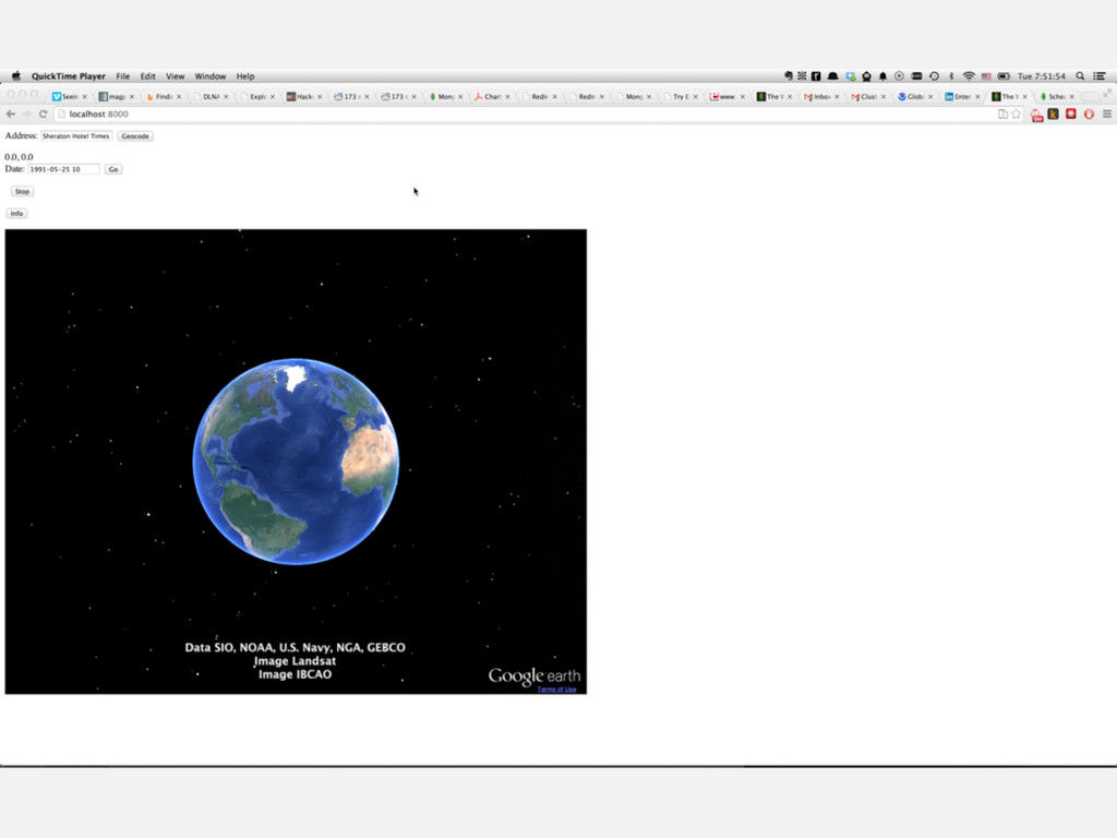
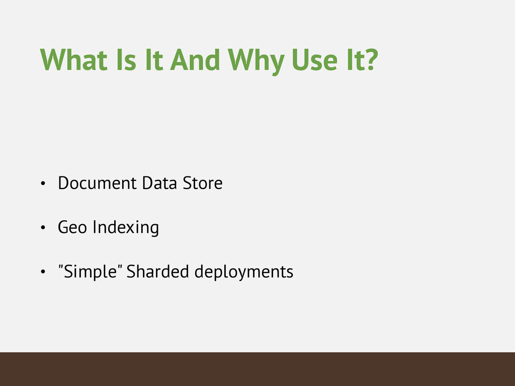
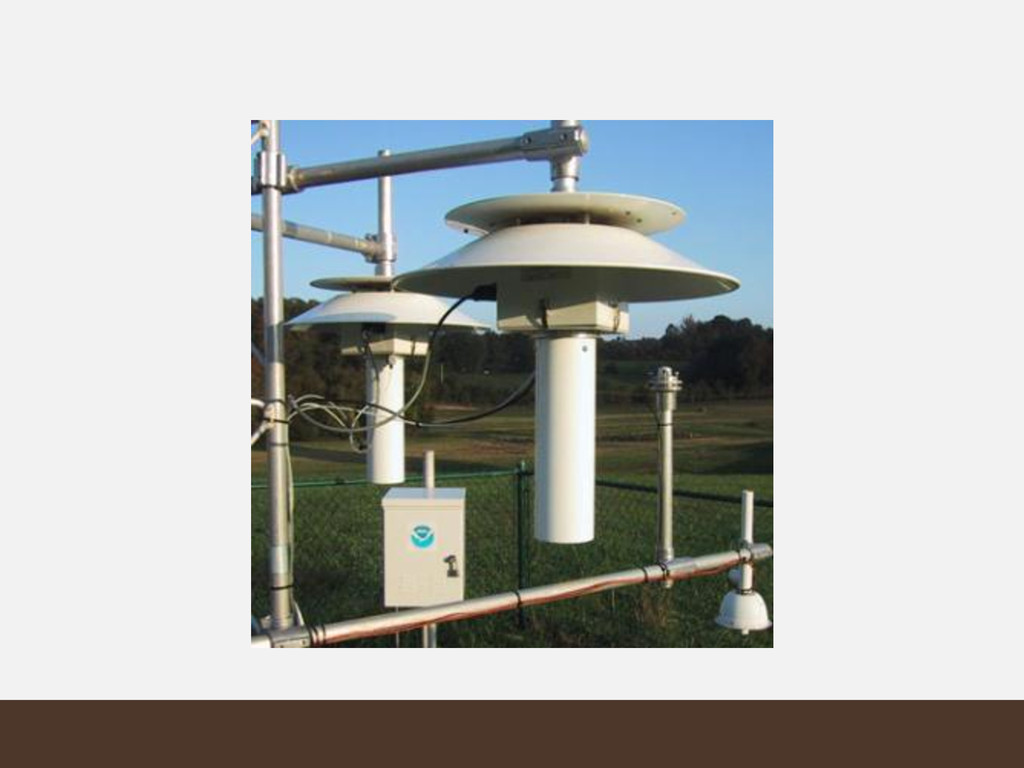
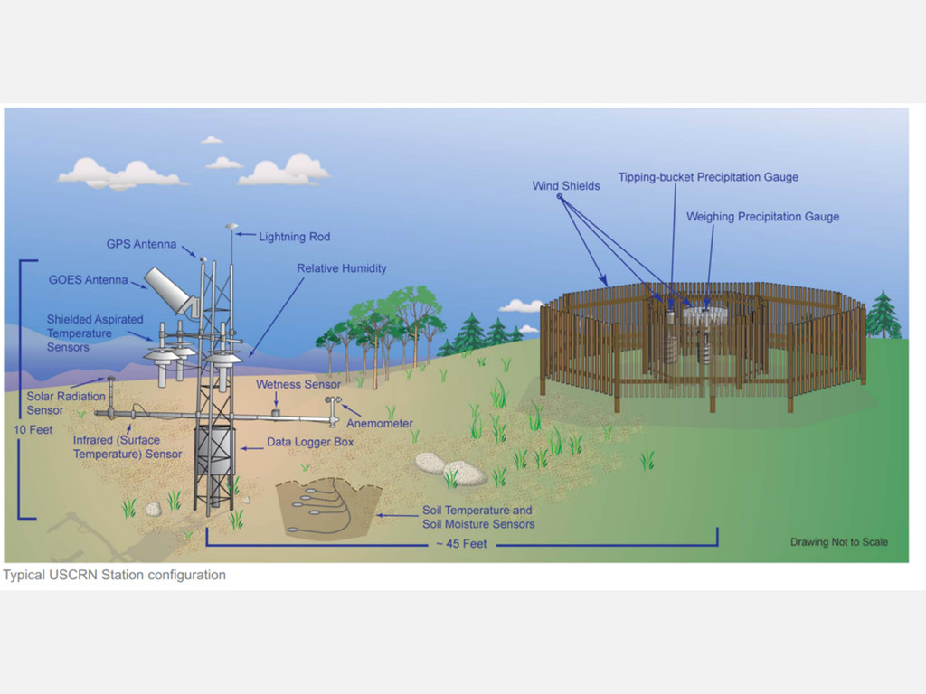
The weather is everywhere and always. That makes for a lot of data. This talk will walk you through how you can use MongoDB to store and analyze worldwide weather data from the entire 20th century in a graphical application. You'll learn how to ask and answer questions about capacity planning and scaling for both real-time and ad-hoc operations when dealing with huge datasets.

Transcript

1. Weather of the Century J. Randall Hunt @jrhunt
 Technical Evangelist, Amazon Web Services @pygotham
2. What was the weather the day you were born?
4. Agenda • Data and Schema • Application • Operational Concerns
5. MONGODB INTERLUDE!
6. What Is It And Why Use It? • Document Data Store • Geo Indexing • "Simple" Sharded deployments
7. Terminology RDBMS MongoDB (Document Store) Database Database Table Collection Row(s) (bson) Document Index Index Join Nope.
8. The Data
9. Where To Get Data?
12. A Weather Datum • A station ID • A timestamp • Lat, Long, Elevation • A LOT OF WEATHER DATA (135 page manual for parsing) • Lots of optional sections
13. How much of it do we have? • 2.5 billion distinct data points • 4 Terabytes • Number of documents is huge, overall data size is reasonable • We'll call this: "moderately big" data
14. How does it grow?
15. How does it grow?
16. Who Else Is This Relevant For? • Particle Physics • Stocks, high frequency trading • Insurance • People with lots of small pieces data
17. Schema Design 101
18. Things We Care About • Performance ‣ Ingestion ‣ App Specific ‣ Ad-hoc • Cost • Flexibility
19. Performance Breakdown • Bulk Loading • Latency and throughput for queries • point in space-time • one station, one year • the whole world at one time • Aggregation and Exploration • warmest and coldest day ever, average temperature, etc.
20. 0303725053947282013060322517+40779-073969FM-15+0048KNYC V0309999C00005030485MN0080475N5+02115+02005100975 ADDAA101000095AU100001015AW1105GA1025+016765999GA2045+024385999 GA3075+030485999GD11991+0167659GD22991+0243859GD33991+0304859... { "st" : "u725053", "ts" : ISODate("2013-06-03T22:51:00Z"), "airTemperature" : { "value" : 21.1, "quality" : "5" }, "atmosphericPressure" : { "value" : 1009.7, "quality" : "5" } } Station ID: NYC Central Park
21. Schema {! st: "u724463",! ts: ISODate("1991-01-01T00:00:00Z"),! position: {! type: "Point",! coordinates: [! -94.6,! 39.117! ]! },! elevation: 231,! … other fields …! }! station ID and source
22. Stations • USAF and WBAN IDs exist for most of North America. Prefix with "u" and "w" then the ID • For ships we use the prefix "x" and their lat and lng to create a station id.
23. Schema {! st: "u724463",! ts: ISODate("1991-01-01T00:00:00Z"),! position: {! type: "Point",! coordinates: [! -94.6,! 39.117! ]! },! elevation: 231,! … other fields …! }! GeoJSON
24. GeoJSON • A rich geographical data format • Lines, MultiLines, Polygons, Geometries • Able to perform queries on complex structures
25. Schema ! airTemperature: {! value: -4.9,! quality: "1"! }!
26. Choice: Embedding? Problem: ~100 "weather codes" and optional sections • Store them inline • Store them in another collection
27. Choice: Embedding? • Embedding keeps your logic in the schema instead of the application. • Depends on cardinality, don't embed "squillions" • Don't embed objects that have to change frequently.
28. Choice: Unique Identifier {_id: ObjectId("53a33f823ed4ac438f8c63b7")}! • Simple, guaranteed unique identifier • 12 bytes
29. Choice: Unique Identifier ! {_id: {! 'st': 'w12345',! 'ts': ISODate("2014-06-19T19:53:58.680Z")! }! } • Not great if there are duplicates • Slightly More complex queries • ~12 bytes saved per document
30. Choice: Field Shortening • Indexes are still the same size • Decreases readability • In our example you can save ~40% space with minimum field lengths • Probably better to go for semi-readable with ~20% space savings
31. {! "_id": ObjectId("5298c40f3004e2fe02922e29"),! "st": "w13731",! "ts": ISODate("1949-01-01T05:00:00Z"),! "airTemperature": {! "quality": "5",! "value": 1.1! },! "skyCondition": {! "cavok": "N",! "ceilingHeight": {! "determination": "9",! "quality": "4",! "value": 1433! }! },! ... ... ...! }! 1236 Bytes
32. {! "_id": ObjectId("5398c40f3004e2fe02922e29"),! "st": "w13731",! "ts": ISODate("1949-01-01T05:00:00Z"),! "aT": {! "q": "5",! "v": 1.1! },! "sC": {! "c": "N",! "cH": {! "d": "9",! "q": "4",! "v": 1433! }! },! ... ... ...! }! 786 Bytes
33. Choice: Indexes • Prefer sparse indexes! All Geo indexes are sparse. • Relying on index intersection can reduce storage needs but compound indexes are more performant. • Build indexes AFTER ingesting the data!
34. The Application
35. Overview Javascript ! Chrome ! Google Earth browser plugin KML ! Python PyMongo Data Data Client Server
36. Aggregation pipeline = [{! '$match': {! 'ts': {! '$gte': dt,! '$lt': dt + timedelta(hours=1)},! 'airTemperature.quality': {! '$in': ['0', '1', '5', '9']}! }! }, {! '$group': {! '_id': '$st',! 'position': {'$first': '$position'},! 'airTemperature': {'$first': '$airTemperature'}}! }]! ! cursor = db.data.aggregate(pipeline, cursor={})!
39. {! name : "New York",! ! geometry : {! type: "MultiPolygon",! coordinates: [! [! [-71.94, 41.28],! [-71.92, 41.29],! /* 2000 more points... */! [-71.94, 41.28]! ]! ]! }! }! db.states.createIndex({! geometry: '2dsphere'! });! GeoFencing
40. GeoFencing db.states.find_one({! 'geometry': {! '$geoIntersects': {! '$geometry': {! 'type': 'Point',! 'coordinates': [lng, lat]}}}})!
41. Operational Concerns
42. Single Server Application mongod i2.8xlarge 251 GB RAM 6 TB SSD c3.8xlarge
43. Sharded Cluster Application / mongos ... 100 x r3.2xlarge 61 GB RAM @ 100 GB disk mongod c3.8xlarge
44. Cost? .. $60,000 / yr $700,000 / yr
45. Performance Breakdown • Bulk Loading • Latency and throughput for queries • point in space-time • one station, one year • the whole world at one time • Aggregation and Exploration • warmest and coldest day ever, average temperature, etc.
46. Bulk Loading: Single Server 8 threads 100 batch size
47. Bulk Loading: Single Server Settings 8 Threads 100 Batch Size Total loading time: 10 h 20 min Documents per second: ~70,000 Index build time 7 h 40 min (ts_1_st_1)
48. Bulk Loading: Sharded Cluster 144 threads
 200 batch size
49. Bulk Loading: Sharded Cluster Shard Key Station ID, hashed Settings 10 mongos @ 144 threads 200 batch size Total loading time: 3 h 10 min Documents per second: ~228,000 Index build time 5 min (ts_1_st_1)
50. Queries: Point in Space-Time db.data.find({"st" : "u747940",
 "ts" : ISODate("1969-07-16T12:00:00Z")})
51. Queries: Point in Space-Time db.data.find({"st" : "u747940",
 "ts" : ISODate("1969-07-16T12:00:00Z")}) 0 0.5 1 1.5 2 single server cluster ms avg 95th 99th max. throughput: 40,000/s 610,000/s (10 mongos)
52. Queries: One Station, One Year db.data.find({"st" : "u103840",
 "ts" : {"$gte": ISODate("1989-01-01"),
 "$lt" : ISODate("1990-01-01")}})
53. Queries: One Station, One Year db.data.find({"st" : "u103840",
 "ts" : {"$gte": ISODate("1989-01-01"),
 "$lt" : ISODate("1990-01-01")}}) 0 1000 2000 3000 4000 5000 single server cluster ms avg 95th 99th max. throughput: 20/s 430/s (10 mongos) targeted query
54. Queries: The Whole World db.data.find({"ts" : ISODate("2000-01-01T00:00:00Z")})
55. Queries: The Whole World db.data.find({"ts" : ISODate("2000-01-01T00:00:00Z")}) 0 2000 4000 6000 8000 10000 single server cluster ms avg 95th 99th max. throughput: 8/s 310/s (10 mongos) scatter/gather query
56. Analytics: Maximum Temperature db.data.aggregate  ([      {  "$match"  :  {  "airTemperature.quality"  :                                                                    {  "$in"  :  [  "1",  "5"  ]  }  }  },      {  "$group"  :  {  "_id"          :  null,
                                  "maxTemp"  :  {  "$max"  :  
                                                              "$airTemperature.value"  }  }  }   ])     61.8 °C = 143 °F 2 h 30 min Single Server 2 min Cluster
57. Summary: Single Server Pro • Cost Effective • Low latency for single queries Con • Table scans are still slow
58. Summary: Cluster ! Con • High cost ! Pro • High throughput • Very good latency for single queries • Scatter-gather yields significant speed-up • Analytics are possible ! ..
59. Thank You! J. Randall Hunt @jrhunt
 Developer Advocate, MongoDB @pygotham