Work Load Modeling and Work Load Modeler in Performance Testing

This presentation is among the Top 27 Best Papers/Practice/Tutorials selected, out of 460+ submissions received, to be presented @STC 2012.

Presentation Abstract

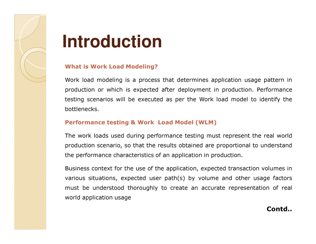
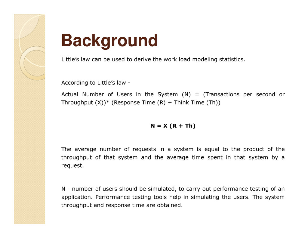
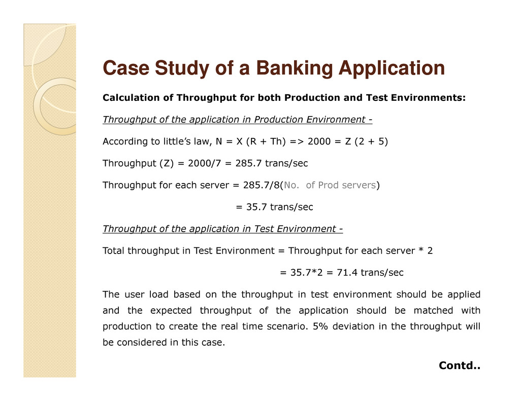
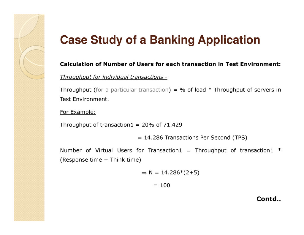
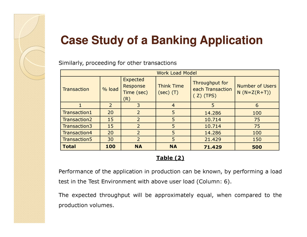
The objective of creating a work load model (WLM) is to make sure that a real-time scenario for the system or application under test (AUT) is created. Accurate predictions and results can be made about the performance of AUT or system when realistic work load models are simulated.

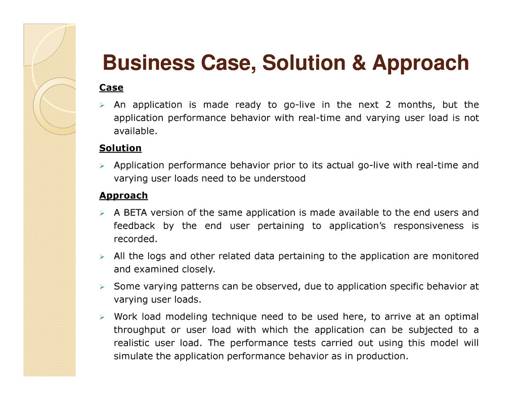
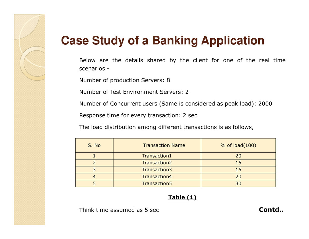
Consider an application, which is made ready to go-live in the next 2 months, but the application performance behavior with real-time and varying user load is not available. To study the application performance behavior prior to its actual go-live with real-time and varying user loads, a BETA version of the same application is made available to the end users with a provision to provide his/her valuable feedback by the end user pertaining to application’s responsiveness. All the logs and other related data pertaining to the application are monitored and examined closely and the results are obtained. Some varying patterns can be observed, due to application specific behavior at varying user loads. Work load modeling technique need to be used here, to arrive at an optimal throughput or user load with which the application can be subjected to a realistic user load. The performance tests carried out using this work load model will simulate the application performance behaviour as in production or after go-live.

About the Author

Amith Kumar Arangi, BE, is currently working as a Test Analyst at Infosys Limited, Hyderabad (NASDAQ: Infy www.infosys.com), He has over 4.5 years of IT experience in manual and performance testing. He received his Bachelors in Electrical & Electronics Engineering from Andhra University in 2008. He has written a number of articles related to Performance testing.

Suresh Suru, BE, is currently working as a Test Analyst at Infosys Limited, Hyderabad (NASDAQ: Infy www.infosys.com), He has over 4.3 years of IT experience in performance testing. He received his Bachelors in Electrical & Electronics Engineering from Osmania University in 2008. He has given presentations and written number of articles related to Performance testing.

Transcript

1. Work Load Modeling and Work Work Load Modeling and Work Load Modeler in Performance Load Modeler in Performance Testing Testing
2. Business Business Case, Solution & Approach Case, Solution & Approach Case An application is made ready to go-live in the next 2 months, but the application performance behavior with real-time and varying user load is not available. Solution Application performance behavior prior to its actual go-live with real-time and varying user loads need to be understood Approach Approach A BETA version of the same application is made available to the end users and feedback by the end user pertaining to application’s responsiveness is recorded. All the logs and other related data pertaining to the application are monitored and examined closely. Some varying patterns can be observed, due to application specific behavior at varying user loads. Work load modeling technique need to be used here, to arrive at an optimal throughput or user load with which the application can be subjected to a realistic user load. The performance tests carried out using this model will simulate the application performance behavior as in production.
3. Introduction Introduction What is Work Load Modeling? Work load modeling is a process that determines application usage pattern in production or which is expected after deployment in production. Performance testing scenarios will be executed as per the Work load model to identify the bottlenecks. Performance testing & Work Load Model (WLM) Performance testing & Work Load Model (WLM) The work loads used during performance testing must represent the real world production scenario, so that the results obtained are proportional to understand the performance characteristics of an application in production. Business context for the use of the application, expected transaction volumes in various situations, expected user path(s) by volume and other usage factors must be understood thoroughly to create an accurate representation of real world application usage Contd..
4. Introduction Introduction Why, WLM is required? Work load modeling is mandatory to make sure that the calculated user load or throughput in the test environment represents an equivalent (scaled down) of production environment. Throughput in production environment can be calculated using the number of users using the application during peak usage, peak usage duration, response times of transactions in the peak usage duration and think time in production times of transactions in the peak usage duration and think time in production environment. Work load model also captures the transaction distribution, load distribution and load pattern.
5. Background Background Little’s law can be used to derive the work load modeling statistics. According to Little’s law - Actual Number of Users in the System (N) = (Transactions per second or Throughput (X))* (Response Time (R) + Think Time (Th)) N = X (R + Th) The average number of requests in a system is equal to the product of the throughput of that system and the average time spent in that system by a request. N - number of users should be simulated, to carry out performance testing of an application. Performance testing tools help in simulating the users. The system throughput and response time are obtained.
6. Work Load Modeling Work Load Modeling - - Approach Approach Identify the critical scenarios for the application from a performance perspective. This should be done as a part of the requirements analysis stage. Identify the set of operations/scenarios performed on the application by an average user. For each of the identified scenarios the following inputs should be captured: ◦ Number of Users using the application in peak hour: The total number of concurrent and simultaneous users accessing the application in a given time frame. ◦ Patterns of requests: A given load of concurrent users may be performing different tasks using the application. Patterns of requests identify the average load of users, and the rate of requests for a given functionality of an application. ◦ Think Time: The user views the information displayed on a page or enters details such as personal details, depending on the nature of action being performed during this time. It varies depending on the complexity of the data on a page. ◦ Response time SLA of transactions in that peak hour Contd..
7. Work Load Modeling Work Load Modeling - - Approach Approach Total number of servers which host the application. Work load model and the transaction load are calculated. Divide the throughput among all the production servers so that the throughput for one single server can be obtained. Scale down the throughput according to the test environment by multiplying the throughput of single server with the number of servers in test environment. Multiply the throughput with the percentage of load to arrive at the final throughput for a particular transaction. Calculate the user load in test environment, using throughput, response time and think time for that particular transaction. Similarly, calculate the user load for all the transactions and perform the load test. The results obtained will give the throughput almost similar to the production environment. NOTE: 5% of deviation will be considered with expected throughput.
8. Different cases Different cases of ‘Work of ‘Work Load Modeling Load Modeling’ ’ Work load modeling (WLM) technique can be applied for variety of cases to arrive at a work load model. The 5 most important and common cases depending upon the data available are identified and work load modeler is designed this to suit for those cases to arrive at the work load model. In all these cases, one needs to identify number of users and throughput in the test environment for a single transaction when the corresponding production data is available Case 1 Case 2 Case 3 Case 4 Case 5
9. Below are the details shared by the client for one of the real time scenarios - Number of production Servers: 8 Number of Test Environment Servers: 2 Number of Concurrent users (Same is considered as peak load): 2000 Response time for every transaction: 2 sec Case Study of a Banking Application Case Study of a Banking Application The load distribution among different transactions is as follows, Table (1) Think time assumed as 5 sec Contd.. S. No Transaction Name % of load(100) 1 Transaction1 20 2 Transaction2 15 3 Transaction3 15 4 Transaction4 20 5 Transaction5 30
10. Case Study of a Banking Application Case Study of a Banking Application Calculation of Throughput for both Production and Test Environments: Throughput of the application in Production Environment - According to little’s law, N = X (R + Th) => 2000 = Z (2 + 5) Throughput (Z) = 2000/7 = 285.7 trans/sec Throughput for each server = 285.7/8(No. of Prod servers) = 35.7 trans/sec Throughput of the application in Test Environment - Total throughput in Test Environment = Throughput for each server * 2 = 35.7*2 = 71.4 trans/sec The user load based on the throughput in test environment should be applied and the expected throughput of the application should be matched with production to create the real time scenario. 5% deviation in the throughput will be considered in this case. Contd..
11. Case Study of a Banking Application Case Study of a Banking Application Calculation of Number of Users for each transaction in Test Environment: Throughput for individual transactions - Throughput (for a particular transaction) = % of load * Throughput of servers in Test Environment. For Example: Throughput of transaction1 = 20% of 71.429 = 14.286 Transactions Per Second (TPS) Number of Virtual Users for Transaction1 = Throughput of transaction1 * (Response time + Think time) ⇒ N = 14.286*(2+5) = 100 Contd..
12. Similarly, proceeding for other transactions Case Study of a Banking Application Case Study of a Banking Application Work Load Model Transaction % load Expected Response Time (sec) (R) Think Time (sec) (T) Throughput for each Transaction ( Z) (TPS) Number of Users N (N=Z(R+T)) 1 2 3 4 5 6 Transaction1 20 2 5 14.286 100 Transaction2 15 2 5 10.714 75 Table (2) Performance of the application in production can be known, by performing a load test in the Test Environment with above user load (Column: 6). The expected throughput will be approximately equal, when compared to the production volumes. Transaction2 15 2 5 10.714 75 Transaction3 15 2 5 10.714 75 Transaction4 20 2 5 14.286 100 Transaction5 30 2 5 21.429 150 Total 100 NA NA 71.429 500
13. Work Load Modeler Work Load Modeler A work load modeler using excel macro is developed, which will calculate the work load (Number of Users or Throughput) for an application under test (AUT) or system. The work load modeler will save time and reduce manual work. Manual calculations in the above example takes lot of time to come up with final numbers. Manual effort is reduced using the work load modeler macro, which will automatically calculate all the Throughput or Number of Users. will automatically calculate all the Throughput or Number of Users. Please find below Work Load Modeler Contd.. Microsoft Excel Macro-Enabled Worksheet
14. Work Load Modeler Work Load Modeler Working with ‘Work Load Modeler’ Microsoft Excel 2003 or above version are required, to work with this work load modeler. Note: 1. In case of Microsoft Excel 2007, make sure that the macros are enabled with the help of macro settings or options. 2. In case of Microsoft Excel 2010, make sure to save this file with .xlsm (Microsoft Excel Macro-Enabled Workbook) extension. Please follow the below steps to run the work load modeler: 1. Open the file and make sure that macros are enabled 2. Enter the data as per the cases (data availability) above, in the “Basic Data” sheet Contd..
15. Work Load Modeler Work Load Modeler Example: Parameter - (Value) *Number of Servers in Production Environment - (8) **Throughput in Production Environment - (10000000) **Number of business days considered for 'Throughput' in Prod - (2) **Number of business hours considered in a business day - (8) (And/or) **Peak Usage Percentage (Throughput) - (30) **Peak Usage Duration considered (Hours) - (2) (And/or) **Number of Concurrent Users in Production - (2000) (Or) Contd..
16. Work Load Modeler Work Load Modeler **Peak Time Production Throughput - (100000) **Peak Time Duration (Hours) - (2) *Number of Transactions under consideration - (10) *Number of Servers in Test Environment - (2) *Response time for every transaction (Sec) - (2) *Think time to be assumed for every transaction (Sec) - (3) *Think time to be assumed for every transaction (Sec) - (3) Note: * denotes a mandatory field whereas ** denotes a case specific field 3. Click on ‘Submit’ button 4. The work load model for the specified case will be obtained in the sheet “WLM”
17. Benefits of Work Load Modeling and Benefits of Work Load Modeling and Work Load Work Load Modeler Modeler Work load Modeling is – Useful to identify business critical transactions and their usage pattern. Useful to replicate a scaled-down version of production. Useful to simulate realistic scenarios. Simple and efficient because it is based on simple operational laws. Platform and environment independent. Platform and environment independent. Work load modeler – Useful to calculate the user load or throughput. Saves time and reduces manual effort. Useful to handle all types of realistic scenarios.
18. References References http://msdn.microsoft.com/en-us/library/bb924367.aspx http://perftesting.codeplex.com/
19. Thank You Amith Kumar Arangi Suresh Suru
20. Case 1 Case 1 When only the below parameters are available. Throughput in production Number of business days for which the throughput is observed Number of application servers in production environment Number of application servers in test environment Number of transactions under consideration Number of transactions under consideration Expected response time. Expected think time.
21. Case 2 Case 2 When only the below parameters are available. Throughput in production Number of business days for which the throughput is observed Percentage distribution of throughput for each scenario. Number of hours for which the percentage distribution is considered. Number of application servers in production environment Number of application servers in production environment Number of application servers in test environment Number of transactions under consideration Expected response time. Expected think time.
22. Case Case 3 3 When only the below parameters are available. Percentage distribution of throughput for each scenario. Number of hours for which the percentage distribution is considered. Number of concurrent users in production. Number of application servers in production environment Number of application servers in test environment Number of application servers in test environment Number of transactions under consideration Expected response time. Expected think time.
23. Case Case 4 4 When only the below parameters are available. Number of concurrent users in production. Number of application servers in production environment Number of application servers in test environment Number of transactions under consideration Expected response time. Expected response time. Expected think time.
24. Case Case 5 5 When only the below parameters are available. Peak time production throughput Peak time duration considered for the peak time production throughput Number of application servers in production environment Number of application servers in test environment Number of transactions under consideration Number of transactions under consideration Expected response time. Expected think time.