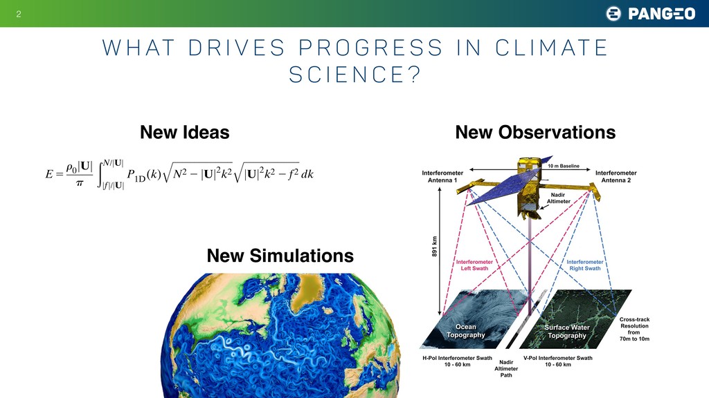
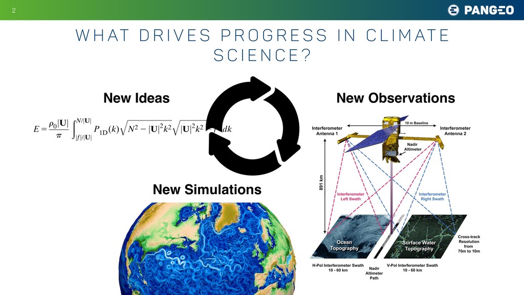
P r o g r e s s i n C l i m at e S c i e n c e ? New Ideas E 5 r 0 jUj p ðN/jUj jfj/jUj P 1D (k ) ffiffiffiffiffiffiffiffiffiffiffiffiffiffiffiffiffiffiffiffiffiffiffiffiffi ffi N2 2 jUj2k 2 q ffiffiffiffiffiffiffiffiffiffiffiffiffiffiffiffiffiffiffiffiffiffiffiffi jUj2k 2 2 f2 q dk , (3) where k 5 (k , l) is now the wavenumber in the reference frame along and across the mean flow U and P 1D (k ) 5 1 2p ð1‘ 2‘ jk j jkj P 2D (k , l) dl (4) is the effective one-dimensional (1D) topographic spectrum. Hence, the wave radiation from 2D topogra- phy reduces to an equivalent problem of wave radiation from 1D topography with the effective spectrum given by P1D (k ). The effective 1D spectrum captures the effects of 2D c. Bottom topography Simulations are configured with multiscale topogra- phy characterized by small-scale abyssal hills a few ki- lometers wide based on multibeam observations from Drake Passage. The topographic spectrum associated with abyssal hills is well described by an anisotropic parametric representation proposed by Goff and Jordan (1988): P 2D (k , l) 5 2p H2(m 2 2) k 0 l 0 1 1 k 2 k 2 0 1 l2 l2 0 !2m/2 , (5) where k 0 and l0 set the wavenumbers of the large hills, m is the high-wavenumber spectral slope, related to the pa- FIG. 3. Averaged profiles of (left) stratification (s21) and (right) flow speed (m s21) in the bottom 2 km from observations (gray), initial condition in the simulations (black), and final state in 2D (blue) and 3D (red) simulations.
P r o g r e s s i n C l i m at e S c i e n c e ? New Ideas New Observations E 5 r 0 jUj p ðN/jUj jfj/jUj P 1D (k ) ffiffiffiffiffiffiffiffiffiffiffiffiffiffiffiffiffiffiffiffiffiffiffiffiffi ffi N2 2 jUj2k 2 q ffiffiffiffiffiffiffiffiffiffiffiffiffiffiffiffiffiffiffiffiffiffiffiffi jUj2k 2 2 f2 q dk , (3) where k 5 (k , l) is now the wavenumber in the reference frame along and across the mean flow U and P 1D (k ) 5 1 2p ð1‘ 2‘ jk j jkj P 2D (k , l) dl (4) is the effective one-dimensional (1D) topographic spectrum. Hence, the wave radiation from 2D topogra- phy reduces to an equivalent problem of wave radiation from 1D topography with the effective spectrum given by P1D (k ). The effective 1D spectrum captures the effects of 2D c. Bottom topography Simulations are configured with multiscale topogra- phy characterized by small-scale abyssal hills a few ki- lometers wide based on multibeam observations from Drake Passage. The topographic spectrum associated with abyssal hills is well described by an anisotropic parametric representation proposed by Goff and Jordan (1988): P 2D (k , l) 5 2p H2(m 2 2) k 0 l 0 1 1 k 2 k 2 0 1 l2 l2 0 !2m/2 , (5) where k 0 and l0 set the wavenumbers of the large hills, m is the high-wavenumber spectral slope, related to the pa- FIG. 3. Averaged profiles of (left) stratification (s21) and (right) flow speed (m s21) in the bottom 2 km from observations (gray), initial condition in the simulations (black), and final state in 2D (blue) and 3D (red) simulations.
P r o g r e s s i n C l i m at e S c i e n c e ? New Ideas New Observations E 5 r 0 jUj p ðN/jUj jfj/jUj P 1D (k ) ffiffiffiffiffiffiffiffiffiffiffiffiffiffiffiffiffiffiffiffiffiffiffiffiffi ffi N2 2 jUj2k 2 q ffiffiffiffiffiffiffiffiffiffiffiffiffiffiffiffiffiffiffiffiffiffiffiffi jUj2k 2 2 f2 q dk , (3) where k 5 (k , l) is now the wavenumber in the reference frame along and across the mean flow U and P 1D (k ) 5 1 2p ð1‘ 2‘ jk j jkj P 2D (k , l) dl (4) is the effective one-dimensional (1D) topographic spectrum. Hence, the wave radiation from 2D topogra- phy reduces to an equivalent problem of wave radiation from 1D topography with the effective spectrum given by P1D (k ). The effective 1D spectrum captures the effects of 2D c. Bottom topography Simulations are configured with multiscale topogra- phy characterized by small-scale abyssal hills a few ki- lometers wide based on multibeam observations from Drake Passage. The topographic spectrum associated with abyssal hills is well described by an anisotropic parametric representation proposed by Goff and Jordan (1988): P 2D (k , l) 5 2p H2(m 2 2) k 0 l 0 1 1 k 2 k 2 0 1 l2 l2 0 !2m/2 , (5) where k 0 and l0 set the wavenumbers of the large hills, m is the high-wavenumber spectral slope, related to the pa- FIG. 3. Averaged profiles of (left) stratification (s21) and (right) flow speed (m s21) in the bottom 2 km from observations (gray), initial condition in the simulations (black), and final state in 2D (blue) and 3D (red) simulations.
P r o g r e s s i n C l i m at e S c i e n c e ? New Ideas New Observations E 5 r 0 jUj p ðN/jUj jfj/jUj P 1D (k ) ffiffiffiffiffiffiffiffiffiffiffiffiffiffiffiffiffiffiffiffiffiffiffiffiffi ffi N2 2 jUj2k 2 q ffiffiffiffiffiffiffiffiffiffiffiffiffiffiffiffiffiffiffiffiffiffiffiffi jUj2k 2 2 f2 q dk , (3) where k 5 (k , l) is now the wavenumber in the reference frame along and across the mean flow U and P 1D (k ) 5 1 2p ð1‘ 2‘ jk j jkj P 2D (k , l) dl (4) is the effective one-dimensional (1D) topographic spectrum. Hence, the wave radiation from 2D topogra- phy reduces to an equivalent problem of wave radiation from 1D topography with the effective spectrum given by P1D (k ). The effective 1D spectrum captures the effects of 2D c. Bottom topography Simulations are configured with multiscale topogra- phy characterized by small-scale abyssal hills a few ki- lometers wide based on multibeam observations from Drake Passage. The topographic spectrum associated with abyssal hills is well described by an anisotropic parametric representation proposed by Goff and Jordan (1988): P 2D (k , l) 5 2p H2(m 2 2) k 0 l 0 1 1 k 2 k 2 0 1 l2 l2 0 !2m/2 , (5) where k 0 and l0 set the wavenumbers of the large hills, m is the high-wavenumber spectral slope, related to the pa- FIG. 3. Averaged profiles of (left) stratification (s21) and (right) flow speed (m s21) in the bottom 2 km from observations (gray), initial condition in the simulations (black), and final state in 2D (blue) and 3D (red) simulations.
P r o g r e s s i n C l i m at e S c i e n c e ? New Ideas New Observations New Simulations E 5 r 0 jUj p ðN/jUj jfj/jUj P 1D (k ) ffiffiffiffiffiffiffiffiffiffiffiffiffiffiffiffiffiffiffiffiffiffiffiffiffi ffi N2 2 jUj2k 2 q ffiffiffiffiffiffiffiffiffiffiffiffiffiffiffiffiffiffiffiffiffiffiffiffi jUj2k 2 2 f2 q dk , (3) where k 5 (k , l) is now the wavenumber in the reference frame along and across the mean flow U and P 1D (k ) 5 1 2p ð1‘ 2‘ jk j jkj P 2D (k , l) dl (4) is the effective one-dimensional (1D) topographic spectrum. Hence, the wave radiation from 2D topogra- phy reduces to an equivalent problem of wave radiation from 1D topography with the effective spectrum given by P1D (k ). The effective 1D spectrum captures the effects of 2D c. Bottom topography Simulations are configured with multiscale topogra- phy characterized by small-scale abyssal hills a few ki- lometers wide based on multibeam observations from Drake Passage. The topographic spectrum associated with abyssal hills is well described by an anisotropic parametric representation proposed by Goff and Jordan (1988): P 2D (k , l) 5 2p H2(m 2 2) k 0 l 0 1 1 k 2 k 2 0 1 l2 l2 0 !2m/2 , (5) where k 0 and l0 set the wavenumbers of the large hills, m is the high-wavenumber spectral slope, related to the pa- FIG. 3. Averaged profiles of (left) stratification (s21) and (right) flow speed (m s21) in the bottom 2 km from observations (gray), initial condition in the simulations (black), and final state in 2D (blue) and 3D (red) simulations.
P r o g r e s s i n C l i m at e S c i e n c e ? New Ideas New Observations New Simulations E 5 r 0 jUj p ðN/jUj jfj/jUj P 1D (k ) ffiffiffiffiffiffiffiffiffiffiffiffiffiffiffiffiffiffiffiffiffiffiffiffiffi ffi N2 2 jUj2k 2 q ffiffiffiffiffiffiffiffiffiffiffiffiffiffiffiffiffiffiffiffiffiffiffiffi jUj2k 2 2 f2 q dk , (3) where k 5 (k , l) is now the wavenumber in the reference frame along and across the mean flow U and P 1D (k ) 5 1 2p ð1‘ 2‘ jk j jkj P 2D (k , l) dl (4) is the effective one-dimensional (1D) topographic spectrum. Hence, the wave radiation from 2D topogra- phy reduces to an equivalent problem of wave radiation from 1D topography with the effective spectrum given by P1D (k ). The effective 1D spectrum captures the effects of 2D c. Bottom topography Simulations are configured with multiscale topogra- phy characterized by small-scale abyssal hills a few ki- lometers wide based on multibeam observations from Drake Passage. The topographic spectrum associated with abyssal hills is well described by an anisotropic parametric representation proposed by Goff and Jordan (1988): P 2D (k , l) 5 2p H2(m 2 2) k 0 l 0 1 1 k 2 k 2 0 1 l2 l2 0 !2m/2 , (5) where k 0 and l0 set the wavenumbers of the large hills, m is the high-wavenumber spectral slope, related to the pa- FIG. 3. Averaged profiles of (left) stratification (s21) and (right) flow speed (m s21) in the bottom 2 km from observations (gray), initial condition in the simulations (black), and final state in 2D (blue) and 3D (red) simulations.
P r o g r e s s i n C l i m at e S c i e n c e ? New Ideas New Observations New Simulations E 5 r 0 jUj p ðN/jUj jfj/jUj P 1D (k ) ffiffiffiffiffiffiffiffiffiffiffiffiffiffiffiffiffiffiffiffiffiffiffiffiffi ffi N2 2 jUj2k 2 q ffiffiffiffiffiffiffiffiffiffiffiffiffiffiffiffiffiffiffiffiffiffiffiffi jUj2k 2 2 f2 q dk , (3) where k 5 (k , l) is now the wavenumber in the reference frame along and across the mean flow U and P 1D (k ) 5 1 2p ð1‘ 2‘ jk j jkj P 2D (k , l) dl (4) is the effective one-dimensional (1D) topographic spectrum. Hence, the wave radiation from 2D topogra- phy reduces to an equivalent problem of wave radiation from 1D topography with the effective spectrum given by P1D (k ). The effective 1D spectrum captures the effects of 2D c. Bottom topography Simulations are configured with multiscale topogra- phy characterized by small-scale abyssal hills a few ki- lometers wide based on multibeam observations from Drake Passage. The topographic spectrum associated with abyssal hills is well described by an anisotropic parametric representation proposed by Goff and Jordan (1988): P 2D (k , l) 5 2p H2(m 2 2) k 0 l 0 1 1 k 2 k 2 0 1 l2 l2 0 !2m/2 , (5) where k 0 and l0 set the wavenumbers of the large hills, m is the high-wavenumber spectral slope, related to the pa- FIG. 3. Averaged profiles of (left) stratification (s21) and (right) flow speed (m s21) in the bottom 2 km from observations (gray), initial condition in the simulations (black), and final state in 2D (blue) and 3D (red) simulations.
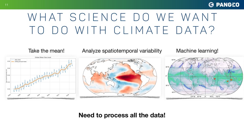
e d o w e w a n t t o d o w i t h C l i m at e d ata? Take the mean! Analyze spatiotemporal variability Machine learning! Need to process all the data!
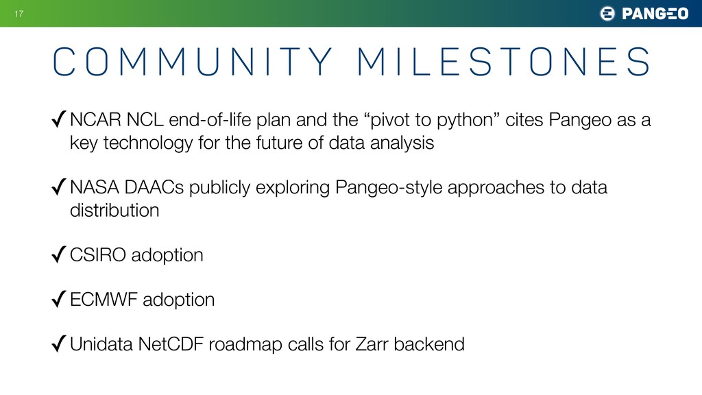
Pangeo as a key technology for the future of data analysis ✓NASA DAACs publicly exploring Pangeo-style approaches to data distribution ✓CSIRO adoption ✓ECMWF adoption ✓Unidata NetCDF roadmap calls for Zarr backend C o m m u n i t y M i l e s t o n e S !16
Pangeo as a key technology for the future of data analysis ✓NASA DAACs publicly exploring Pangeo-style approaches to data distribution ✓CSIRO adoption ✓ECMWF adoption ✓Unidata NetCDF roadmap calls for Zarr backend C o m m u n i t y M i l e s t o n e S !17
Pangeo as a key technology for the future of data analysis ✓NASA DAACs publicly exploring Pangeo-style approaches to data distribution ✓CSIRO adoption ✓ECMWF adoption ✓Unidata NetCDF roadmap calls for Zarr backend C o m m u n i t y M i l e s t o n e S !17
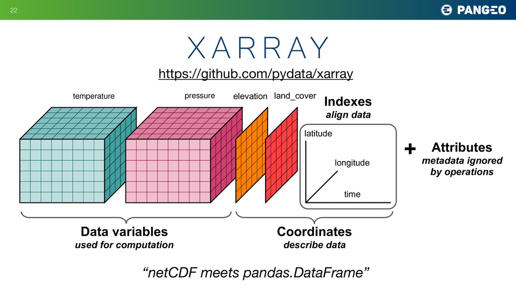
Data variables used for computation Coordinates describe data Indexes align data Attributes metadata ignored by operations + land_cover “netCDF meets pandas.DataFrame” https://github.com/pydata/xarray
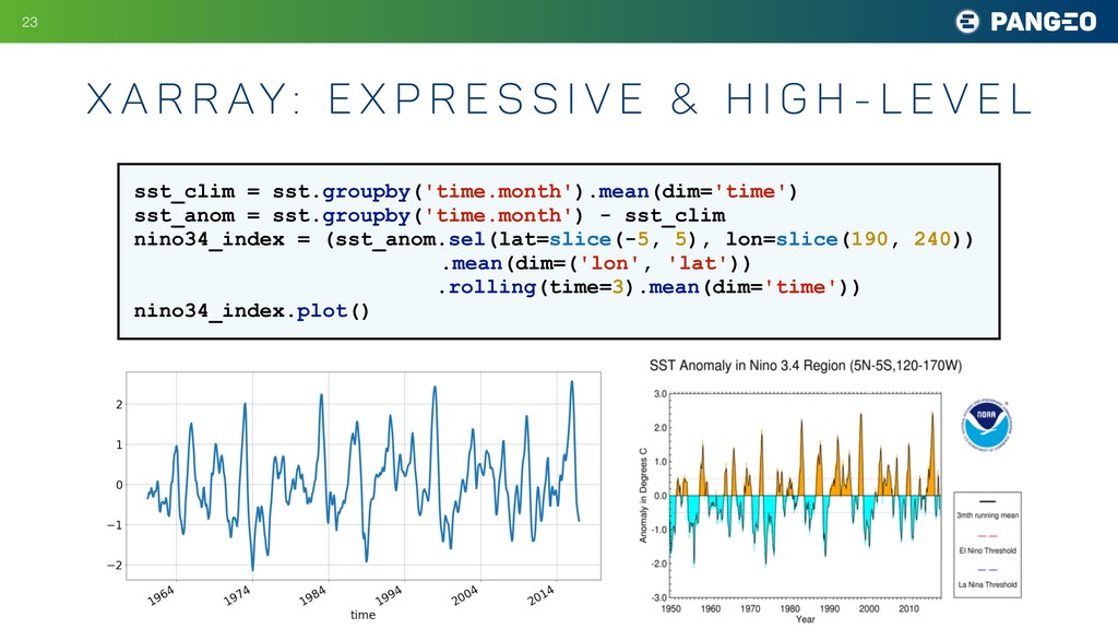
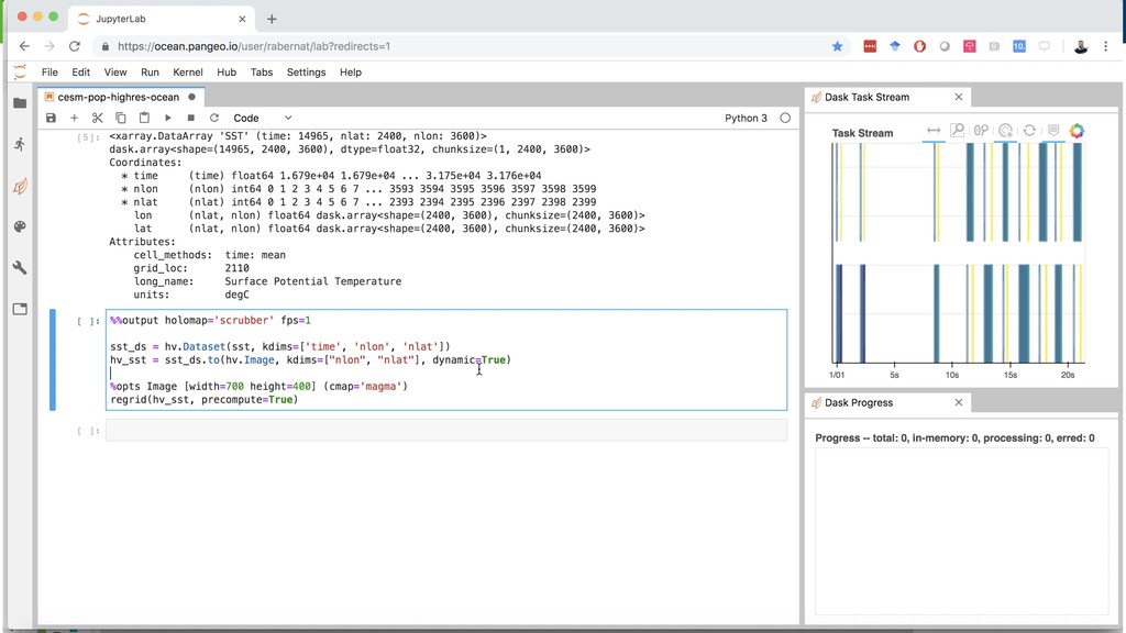
e s s i v e & h i g h - l e v e l !23 sst_clim = sst.groupby('time.month').mean(dim='time') sst_anom = sst.groupby('time.month') - sst_clim nino34_index = (sst_anom.sel(lat=slice(-5, 5), lon=slice(190, 240)) .mean(dim=('lon', 'lat')) .rolling(time=3).mean(dim='time')) nino34_index.plot()
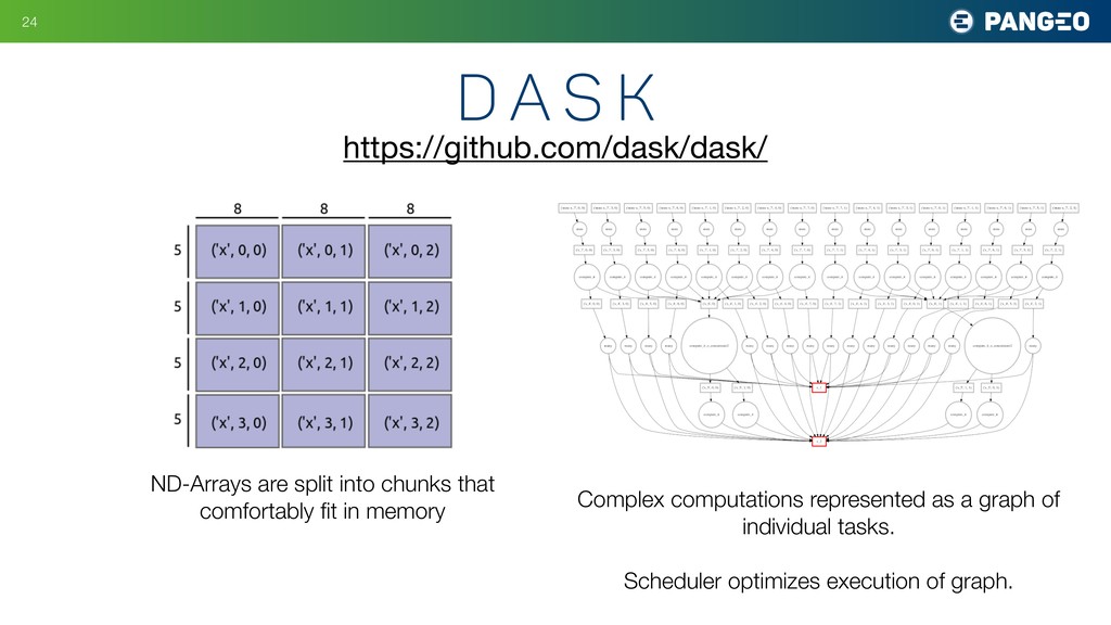
graph of individual tasks. Scheduler optimizes execution of graph. https://github.com/dask/dask/ ND-Arrays are split into chunks that comfortably fit in memory
graph of individual tasks. Scheduler optimizes execution of graph. https://github.com/dask/dask/ ND-Arrays are split into chunks that comfortably fit in memory
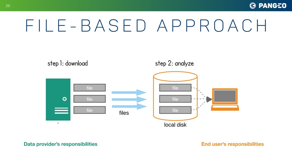
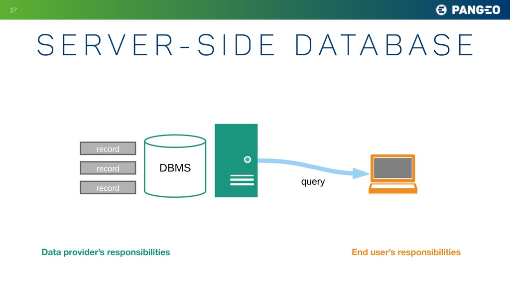
A p p r o a c h !26 a) file-based approach step 1 : dow nload step 2: analyze ` file file file b) database approach file file file local disk files Data provider’s responsibilities End user’s responsibilities
e D ata b a s e !27 ` file file file b) database approach record record record DBMS file file file local disk query c) cloud approach files Data provider’s responsibilities End user’s responsibilities
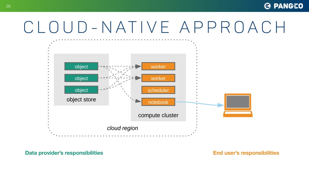
e A p p r o a c h !28 object store record query c) cloud approach object object object cloud region compute cluster worker worker scheduler notebook Data provider’s responsibilities End user’s responsibilities
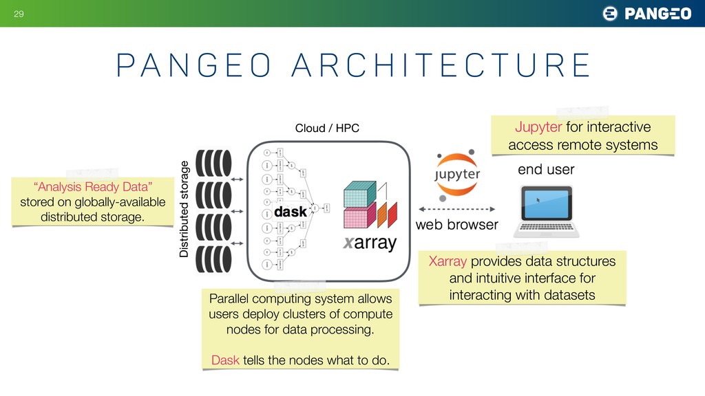
i t e c t u r e Jupyter for interactive access remote systems Cloud / HPC Xarray provides data structures and intuitive interface for interacting with datasets Parallel computing system allows users deploy clusters of compute nodes for data processing. Dask tells the nodes what to do. Distributed storage “Analysis Ready Data” stored on globally-available distributed storage.
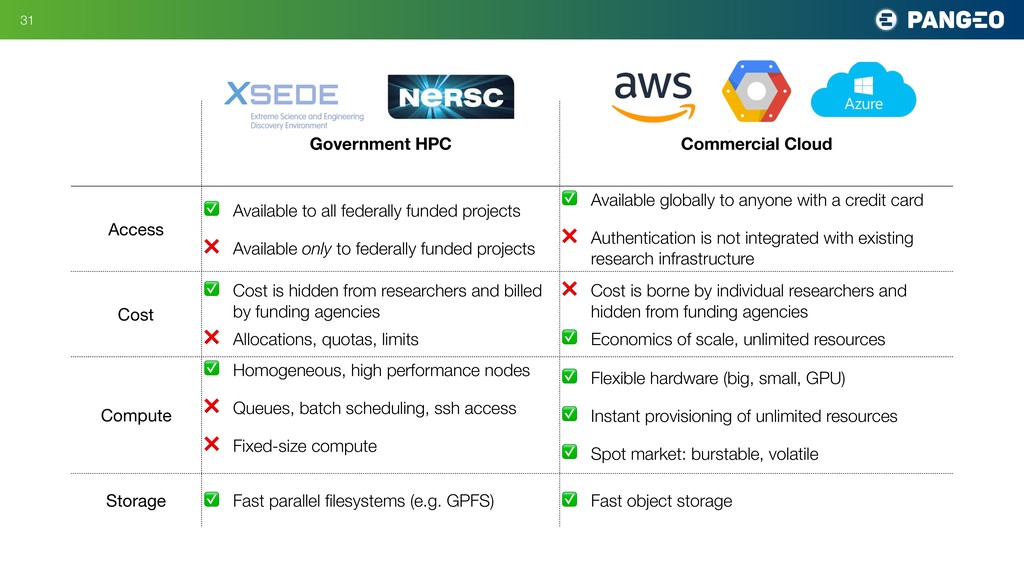
federally funded projects ❌ Available only to federally funded projects ✅ Available globally to anyone with a credit card ❌ Authentication is not integrated with existing research infrastructure Cost ✅ Cost is hidden from researchers and billed by funding agencies ❌ Allocations, quotas, limits ❌ Cost is borne by individual researchers and hidden from funding agencies ✅ Economics of scale, unlimited resources Compute ✅ Homogeneous, high performance nodes ❌ Queues, batch scheduling, ssh access ❌ Fixed-size compute ✅ Flexible hardware (big, small, GPU) ✅ Instant provisioning of unlimited resources ✅ Spot market: burstable, volatile Storage ✅ Fast parallel filesystems (e.g. GPFS) ✅ Fast object storage
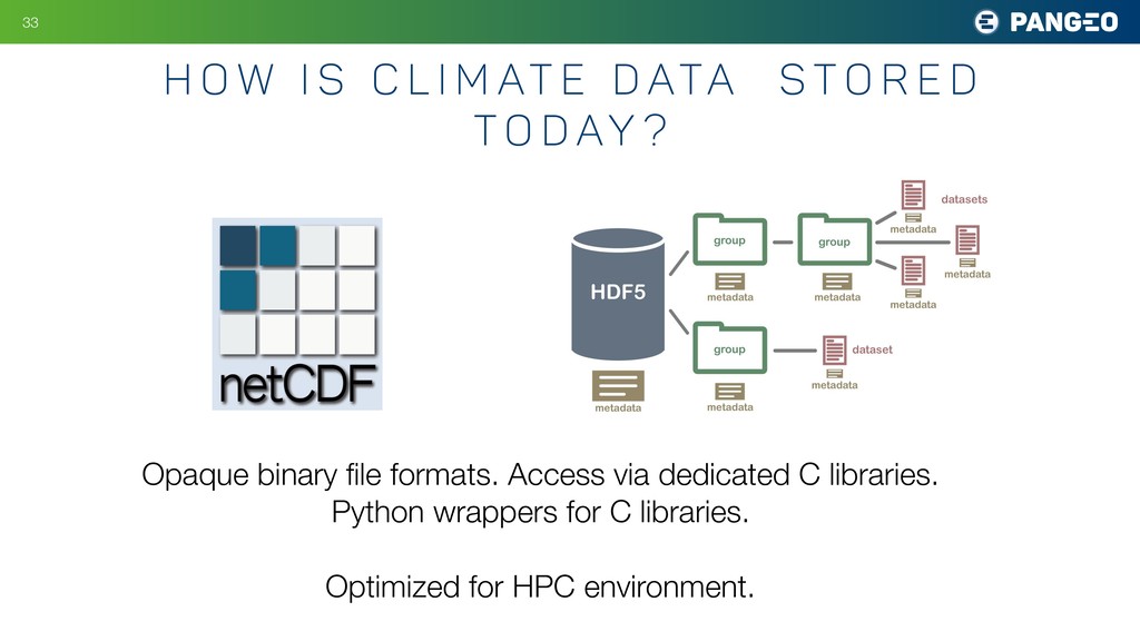
at e d ata s t o r e d t o d ay ? Opaque binary file formats. Access via dedicated C libraries. Python wrappers for C libraries. Optimized for HPC environment.
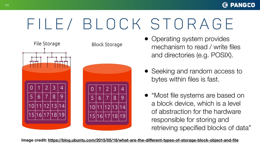
k s t o r a g e Image credit: https://blog.ubuntu.com/2015/05/18/what-are-the-different-types-of-storage-block-object-and-file • Operating system provides mechanism to read / write files and directories (e.g. POSIX). • Seeking and random access to bytes within files is fast. • “Most file systems are based on a block device, which is a level of abstraction for the hardware responsible for storing and retrieving specified blocks of data”
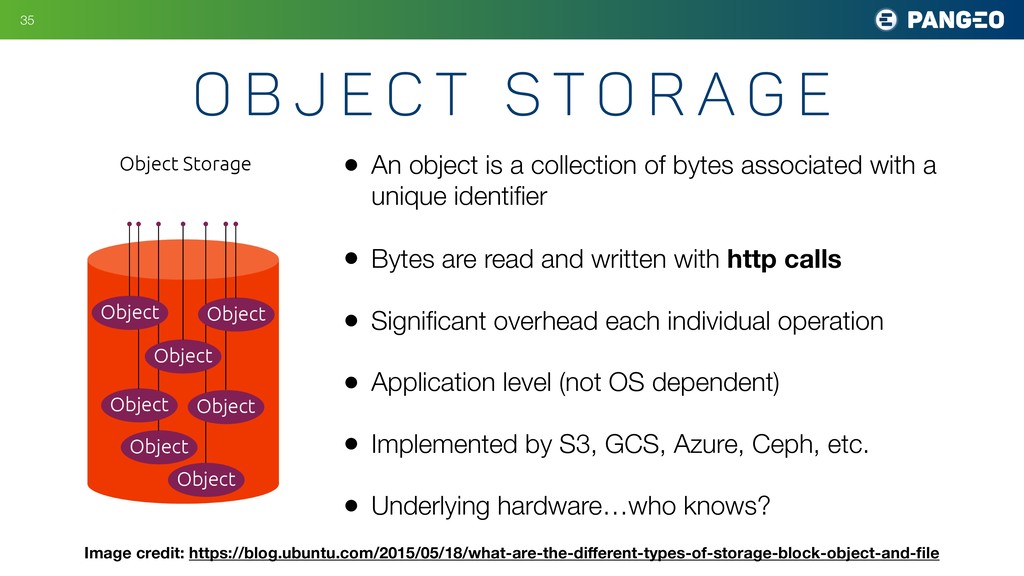
r a g e Image credit: https://blog.ubuntu.com/2015/05/18/what-are-the-different-types-of-storage-block-object-and-file • An object is a collection of bytes associated with a unique identifier • Bytes are read and written with http calls • Significant overhead each individual operation • Application level (not OS dependent) • Implemented by S3, GCS, Azure, Ceph, etc. • Underlying hardware…who knows?
J u s t D u m p o u r N e t C D F F i l e A r c h i v e s i n t o s 3 ? !36 • Can’t issue an HTTP request to peek into an HDF file. HDF client library does not support this*. ➡ if we want to know what’s in it, have to download the whole thing • Most netCDF datasets use very small “granules” (e.g. one netCDF file per day). Pangeo users want to look at the whole dataset. Scanning thousands of HDF files is very expensive in object storage.
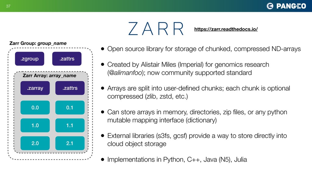
• Created by Alistair Miles (Imperial) for genomics research (@alimanfoo); now community supported standard • Arrays are split into user-defined chunks; each chunk is optional compressed (zlib, zstd, etc.) • Can store arrays in memory, directories, zip files, or any python mutable mapping interface (dictionary) • External libraries (s3fs, gcsf) provide a way to store directly into cloud object storage • Implementations in Python, C++, Java (N5), Julia !37 z a r r Zarr Group: group_name .zgroup .zattrs .zarray .zattrs Zarr Array: array_name 0.0 0.1 2.0 1.0 1.1 2.1 https://zarr.readthedocs.io/
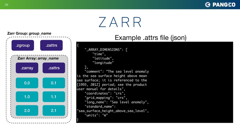
.zarray .zattrs Zarr Array: array_name 0.0 0.1 2.0 1.0 1.1 2.1 { "_ARRAY_DIMENSIONS": [ "time", "latitude", "longitude" ], "comment": "The sea level anomaly is the sea surface height above mean sea surface; it is referenced to the [1993, 2012] period; see the product user manual for details", "coordinates": "crs", "grid_mapping": "crs", "long_name": "Sea level anomaly", "standard_name": "sea_surface_height_above_sea_level", "units": "m" } Example .attrs file (json)
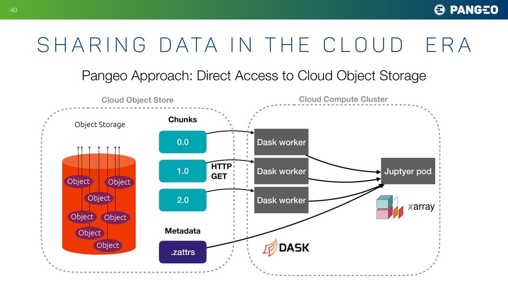
worker Dask worker Juptyer pod S h a r i n g D ata i n t h e C l o u d E R A Pangeo Approach: Direct Access to Cloud Object Storage Cloud Object Store Cloud Compute Cluster HTTP GET
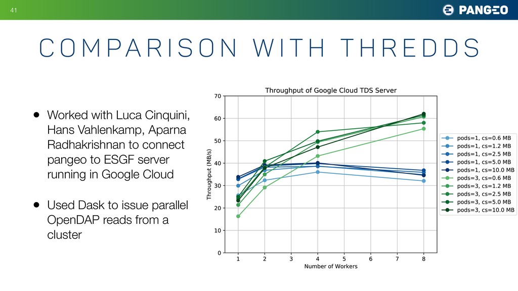
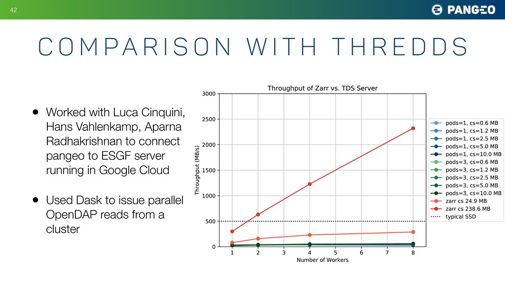
w i t h T H R E D D S • Worked with Luca Cinquini, Hans Vahlenkamp, Aparna Radhakrishnan to connect pangeo to ESGF server running in Google Cloud • Used Dask to issue parallel OpenDAP reads from a cluster
w i t h T H R E D D S • Worked with Luca Cinquini, Hans Vahlenkamp, Aparna Radhakrishnan to connect pangeo to ESGF server running in Google Cloud • Used Dask to issue parallel OpenDAP reads from a cluster
hidden costs. • Legacy data distribution approach: much cheaper per TB But MANY hidden costs • Hardware, bandwidth, IT support, etc. • Data is not accessible to compute, so users have to download it to local “dark replicas”. Huge cost multiplier to funding agencies! • What is the cost of missed science opportunities? !43 C o s t C o n s i d e r at i o n s
• Access an existing Pangeo deployment on an HPC cluster, or cloud resources (http://pangeo.io/deployments.html) • Adapt Pangeo elements to meet your projects needs (data portals, etc.) and give feedback via github: github.com/pangeo-data/pangeo !45 H o w t o g e t i n v o lv e d http://pangeo.io
of our peer institutions. By developing infrastructure collaboratively, we can accomplish much more than any one institution can alone. • Open source - Because infrastructure is code, the code should be licensed in a way that enables the entire research community to reuse and build upon it. • Modular - “all in one” solutions are impossible to maintain long term. Separation of concerns is a key principle of good software and systems engineering. • Vendor neutral - Academic research infrastructure should use only vendor- neutral services APIs. If this principle is followed, it means we can redeploy our infrastructure anywhere. !47 Pa n g e o P r i n c i p l e s f o r C l o u d - N at i v e S c i e n c e I n f r a s t r u c t u r e