Error Correction Over Noisy Channels

A primer on Information Theory and its fundamental theorem which I gave in the spring of 2012 as part of MAT 490 at Berry College. There are a few significant typos in this presentation, so be warned.

Transcript

1. 0 1 0 1 1 1 1 0 0 0 1 1 1 0 0 0 1 1 1 1 1 0 1 1 0 0 1 0 1 1 1 1 1 1 0 0 0 0 Error Correction Over Noisy Channels and the Noisy Channel Coding Theorem Charles Julian Knight Berry College March 20, 2012
2. 0 1 0 1 1 1 1 0 0 0 1 1 1 0 0 0 1 1 1 1 1 0 1 1 0 0 1 0 1 1 1 1 1 1 0 0 0 0 Introduction How do you... • Talk to space shuttles? • Avoid cross-talk over telephone lines? • Make a CD that still plays if you scratch it?
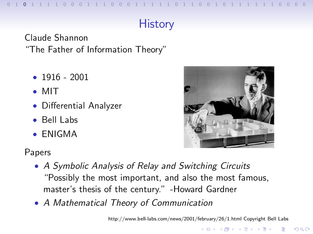
3. 0 1 0 1 1 1 1 0 0 0 1 1 1 0 0 0 1 1 1 1 1 0 1 1 0 0 1 0 1 1 1 1 1 1 0 0 0 0 History Claude Shannon “The Father of Information Theory” • 1916 - 2001 • MIT • Differential Analyzer • Bell Labs • ENIGMA Papers • A Symbolic Analysis of Relay and Switching Circuits “Possibly the most important, and also the most famous, master’s thesis of the century.” -Howard Gardner • A Mathematical Theory of Communication http://www.bell-labs.com/news/2001/february/26/1.html Copyright Bell Labs
4. 0 1 0 1 1 1 1 0 0 0 1 1 1 0 0 0 1 1 1 1 1 0 1 1 0 0 1 0 1 1 1 1 1 1 0 0 0 0 Definitions and Notation • Shannon bit – “The amount of information gained (or entropy removed) upon learning the answer to a question whose two possible answers were equally likely, a priori.”
5. 0 1 0 1 1 1 1 0 0 0 1 1 1 0 0 0 1 1 1 1 1 0 1 1 0 0 1 0 1 1 1 1 1 1 0 0 0 0 Definitions and Notation • Shannon bit – “The amount of information gained (or entropy removed) upon learning the answer to a question whose two possible answers were equally likely, a priori.” • Target Space – {x1, x2, ..., xn}
6. 0 1 0 1 1 1 1 0 0 0 1 1 1 0 0 0 1 1 1 1 1 0 1 1 0 0 1 0 1 1 1 1 1 1 0 0 0 0 Definitions and Notation • Shannon bit – “The amount of information gained (or entropy removed) upon learning the answer to a question whose two possible answers were equally likely, a priori.” • Target Space – {x1, x2, ..., xn} • P(X = x1) or simply P(x1)
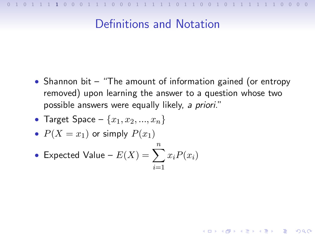
7. 0 1 0 1 1 1 1 0 0 0 1 1 1 0 0 0 1 1 1 1 1 0 1 1 0 0 1 0 1 1 1 1 1 1 0 0 0 0 Definitions and Notation • Shannon bit – “The amount of information gained (or entropy removed) upon learning the answer to a question whose two possible answers were equally likely, a priori.” • Target Space – {x1, x2, ..., xn} • P(X = x1) or simply P(x1) • Expected Value – E(X) = n i=1 xiP(xi)
8. 0 1 0 1 1 1 1 0 0 0 1 1 1 0 0 0 1 1 1 1 1 0 1 1 0 0 1 0 1 1 1 1 1 1 0 0 0 0 Bayes’ Theorem Conditional probability: P(X|Y )
9. 0 1 0 1 1 1 1 0 0 0 1 1 1 0 0 0 1 1 1 1 1 0 1 1 0 0 1 0 1 1 1 1 1 1 0 0 0 0 Bayes’ Theorem Conditional probability: P(X|Y ) P(U|V ) = P(V |U)P(U) P(V )
10. 0 1 0 1 1 1 1 0 0 0 1 1 1 0 0 0 1 1 1 1 1 0 1 1 0 0 1 0 1 1 1 1 1 1 0 0 0 0 Bayes’ Theorem Conditional probability: P(X|Y ) P(U|V ) = P(V |U)P(U) P(V ) = P(UandV ) P(V )
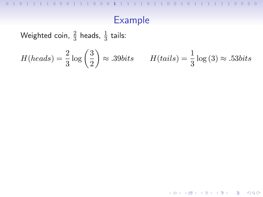
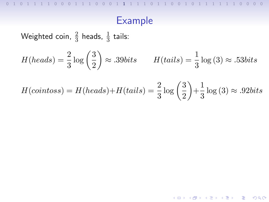
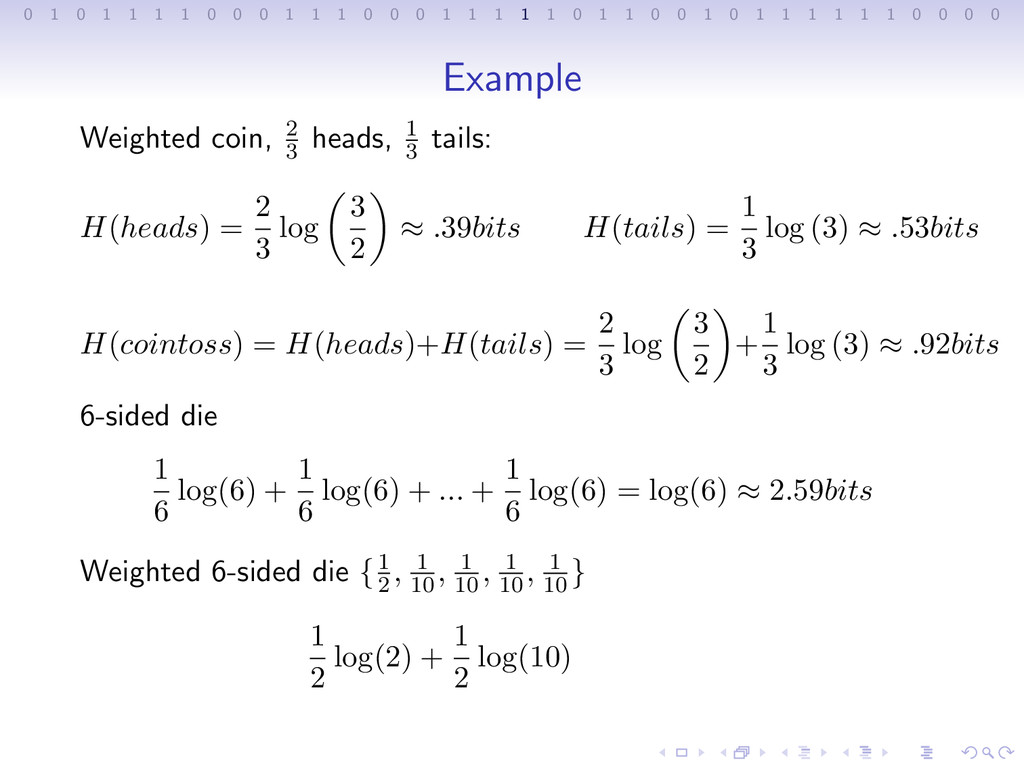
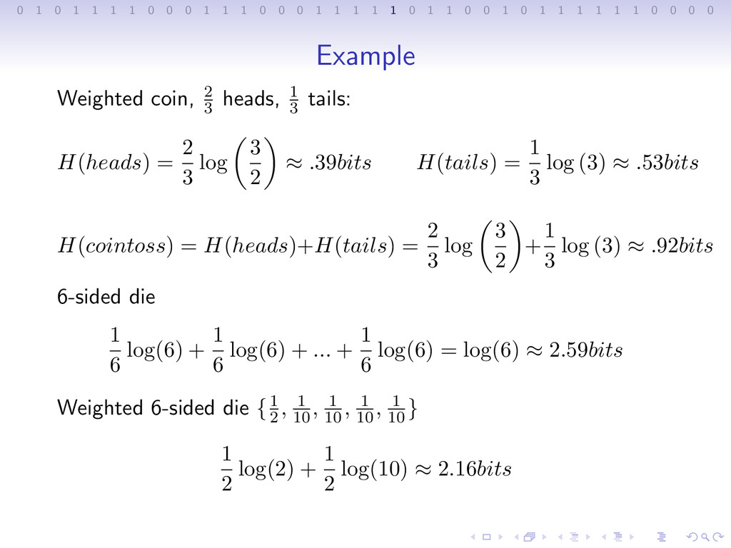
11. 0 1 0 1 1 1 1 0 0 0 1 1 1 0 0 0 1 1 1 1 1 0 1 1 0 0 1 0 1 1 1 1 1 1 0 0 0 0 Shannon Entropy A measure of the amount of uncertainty in the value of a random variable, measured in Shannon bits. Example: Coin Toss
12. 0 1 0 1 1 1 1 0 0 0 1 1 1 0 0 0 1 1 1 1 1 0 1 1 0 0 1 0 1 1 1 1 1 1 0 0 0 0 Shannon Entropy A measure of the amount of uncertainty in the value of a random variable, measured in Shannon bits. Example: Coin Toss Two notes: • Entropy in Thermodynamics
13. 0 1 0 1 1 1 1 0 0 0 1 1 1 0 0 0 1 1 1 1 1 0 1 1 0 0 1 0 1 1 1 1 1 1 0 0 0 0 Shannon Entropy A measure of the amount of uncertainty in the value of a random variable, measured in Shannon bits. Example: Coin Toss Two notes: • Entropy in Thermodynamics • Shannon bits vs. digital bits
14. 0 1 0 1 1 1 1 0 0 0 1 1 1 0 0 0 1 1 1 1 1 0 1 1 0 0 1 0 1 1 1 1 1 1 0 0 0 0 Entropy Function For random variable X with target space x1, x2, ..., xn H(X) = n i=0 P(xi) log2 1 P(xi)
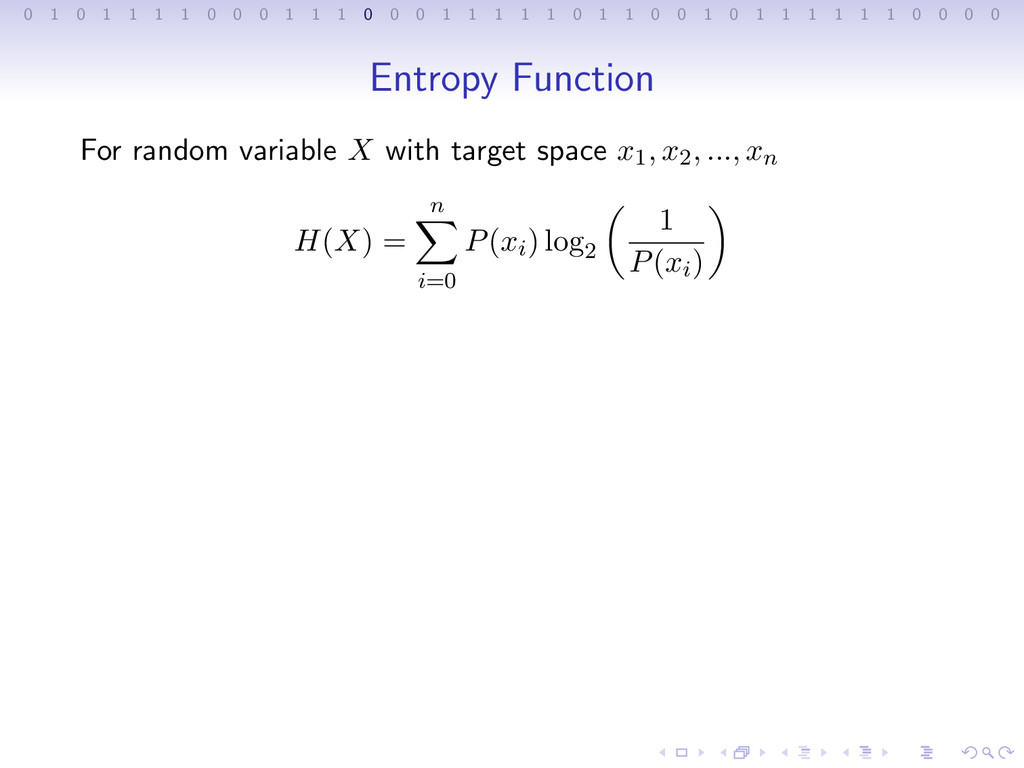
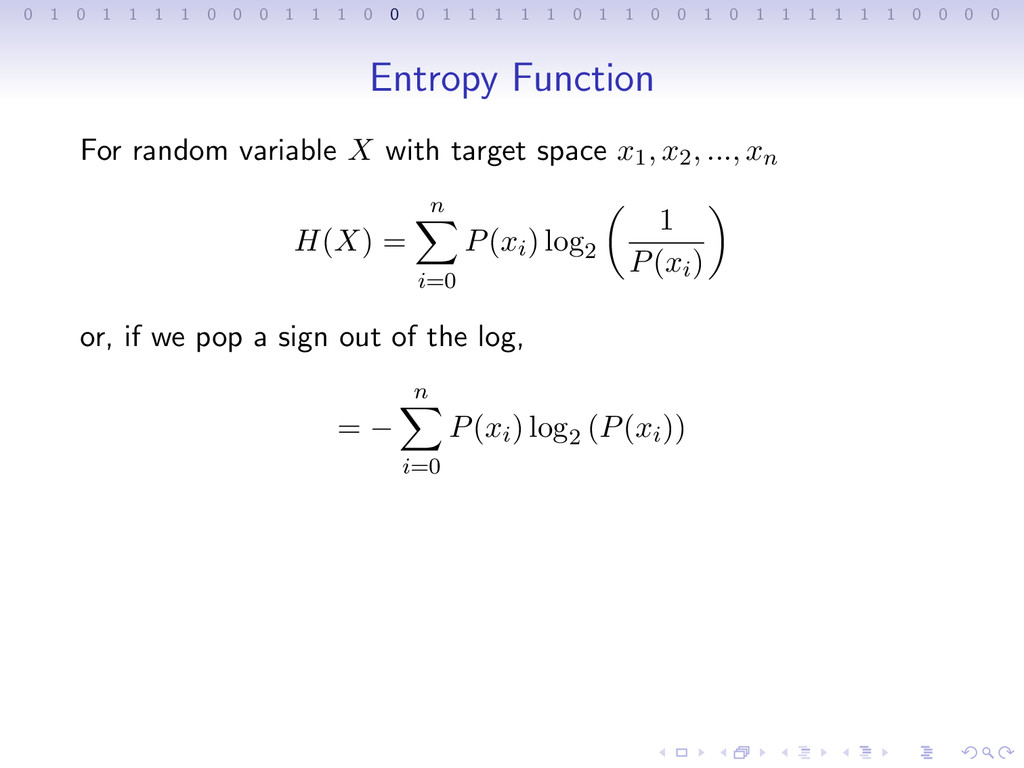
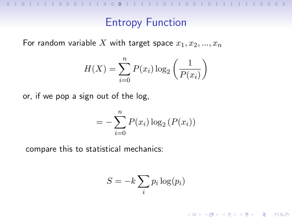
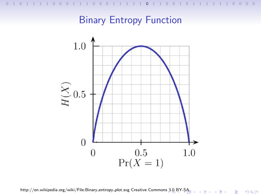
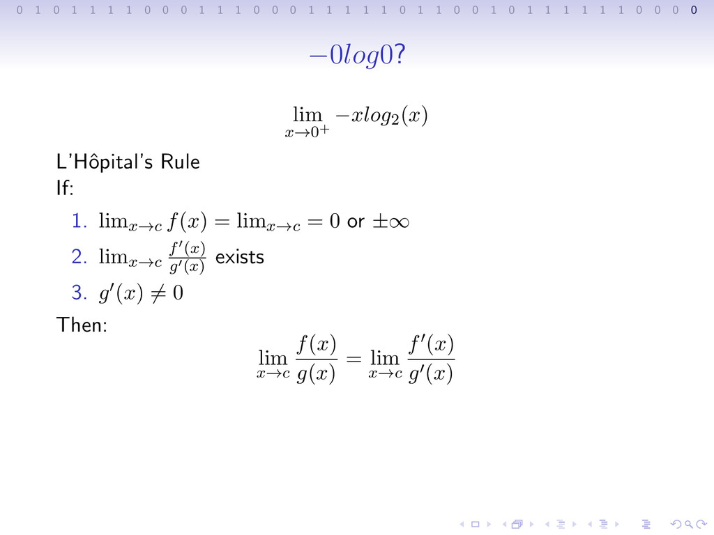
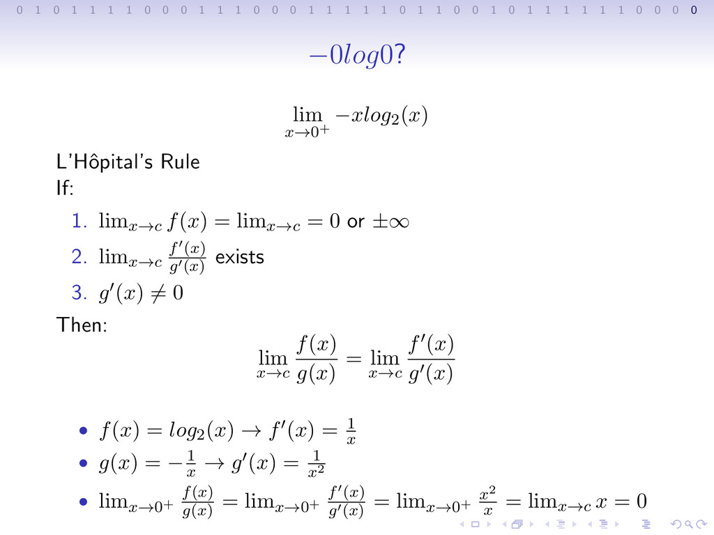
15. 0 1 0 1 1 1 1 0 0 0 1 1 1 0 0 0 1 1 1 1 1 0 1 1 0 0 1 0 1 1 1 1 1 1 0 0 0 0 Entropy Function For random variable X with target space x1, x2, ..., xn H(X) = n i=0 P(xi) log2 1 P(xi) or, if we pop a sign out of the log, = − n i=0 P(xi) log2 (P(xi))
16. 0 1 0 1 1 1 1 0 0 0 1 1 1 0 0 0 1 1 1 1 1 0 1 1 0 0 1 0 1 1 1 1 1 1 0 0 0 0 Entropy Function For random variable X with target space x1, x2, ..., xn H(X) = n i=0 P(xi) log2 1 P(xi) or, if we pop a sign out of the log, = − n i=0 P(xi) log2 (P(xi)) compare this to statistical mechanics: S = −k i pi log(pi)
17. 0 1 0 1 1 1 1 0 0 0 1 1 1 0 0 0 1 1 1 1 1 0 1 1 0 0 1 0 1 1 1 1 1 1 0 0 0 0 Example Weighted coin, 2 3 heads, 1 3 tails: H(heads) = 2 3 log 3 2 ≈ .39bits H(tails) = 1 3 log (3) ≈ .53bits
18. 0 1 0 1 1 1 1 0 0 0 1 1 1 0 0 0 1 1 1 1 1 0 1 1 0 0 1 0 1 1 1 1 1 1 0 0 0 0 Example Weighted coin, 2 3 heads, 1 3 tails: H(heads) = 2 3 log 3 2 ≈ .39bits H(tails) = 1 3 log (3) ≈ .53bits H(cointoss) = H(heads)+H(tails) = 2 3 log 3 2 + 1 3 log (3) ≈ .92bits
19. 0 1 0 1 1 1 1 0 0 0 1 1 1 0 0 0 1 1 1 1 1 0 1 1 0 0 1 0 1 1 1 1 1 1 0 0 0 0 Example Weighted coin, 2 3 heads, 1 3 tails: H(heads) = 2 3 log 3 2 ≈ .39bits H(tails) = 1 3 log (3) ≈ .53bits H(cointoss) = H(heads)+H(tails) = 2 3 log 3 2 + 1 3 log (3) ≈ .92bits 6-sided die 1 6 log(6) + 1 6 log(6) + ... + 1 6 log(6) = log(6) ≈ 2.59bits
20. 0 1 0 1 1 1 1 0 0 0 1 1 1 0 0 0 1 1 1 1 1 0 1 1 0 0 1 0 1 1 1 1 1 1 0 0 0 0 Example Weighted coin, 2 3 heads, 1 3 tails: H(heads) = 2 3 log 3 2 ≈ .39bits H(tails) = 1 3 log (3) ≈ .53bits H(cointoss) = H(heads)+H(tails) = 2 3 log 3 2 + 1 3 log (3) ≈ .92bits 6-sided die 1 6 log(6) + 1 6 log(6) + ... + 1 6 log(6) = log(6) ≈ 2.59bits Weighted 6-sided die {1 2 , 1 10 , 1 10 , 1 10 , 1 10 } 1 2 log(2) + 1 2 log(10)
21. 0 1 0 1 1 1 1 0 0 0 1 1 1 0 0 0 1 1 1 1 1 0 1 1 0 0 1 0 1 1 1 1 1 1 0 0 0 0 Example Weighted coin, 2 3 heads, 1 3 tails: H(heads) = 2 3 log 3 2 ≈ .39bits H(tails) = 1 3 log (3) ≈ .53bits H(cointoss) = H(heads)+H(tails) = 2 3 log 3 2 + 1 3 log (3) ≈ .92bits 6-sided die 1 6 log(6) + 1 6 log(6) + ... + 1 6 log(6) = log(6) ≈ 2.59bits Weighted 6-sided die {1 2 , 1 10 , 1 10 , 1 10 , 1 10 } 1 2 log(2) + 1 2 log(10) ≈ 2.16bits
22. 0 1 0 1 1 1 1 0 0 0 1 1 1 0 0 0 1 1 1 1 1 0 1 1 0 0 1 0 1 1 1 1 1 1 0 0 0 0 Binary Entropy Function http://en.wikipedia.org/wiki/File:Binary entropy plot.svg Creative Commons 3.0 BY-SA
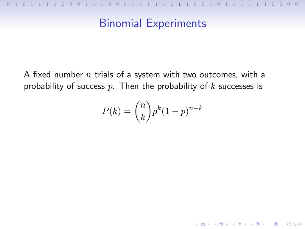
23. 0 1 0 1 1 1 1 0 0 0 1 1 1 0 0 0 1 1 1 1 1 0 1 1 0 0 1 0 1 1 1 1 1 1 0 0 0 0 Binomial Experiments A fixed number n trials of a system with two outcomes, with a probability of success p. Then the probability of k successes is P(k) = n k pk(1 − p)n−k
24. 0 1 0 1 1 1 1 0 0 0 1 1 1 0 0 0 1 1 1 1 1 0 1 1 0 0 1 0 1 1 1 1 1 1 0 0 0 0 Binomial Experiments A fixed number n trials of a system with two outcomes, with a probability of success p. Then the probability of k successes is P(k) = n k pk(1 − p)n−k Binomial coefficient: n! k!(n − k)!
25. 0 1 0 1 1 1 1 0 0 0 1 1 1 0 0 0 1 1 1 1 1 0 1 1 0 0 1 0 1 1 1 1 1 1 0 0 0 0 Noisy Channels • Channel – A medium (physical or logical) over which information is sent.
26. 0 1 0 1 1 1 1 0 0 0 1 1 1 0 0 0 1 1 1 1 1 0 1 1 0 0 1 0 1 1 1 1 1 1 0 0 0 0 Noisy Channels • Channel – A medium (physical or logical) over which information is sent. • Noisy channel – Channel which has some probability (noise parameter f) that a bit will swap values (be “flipped”).
27. 0 1 0 1 1 1 1 0 0 0 1 1 1 0 0 0 1 1 1 1 1 0 1 1 0 0 1 0 1 1 1 1 1 1 0 0 0 0 Noise Simulation By Randall Monroe, xkcd.com/171, Creative Commons 2.5 BY-NC
28. 0 1 0 1 1 1 1 0 0 0 1 1 1 0 0 0 1 1 1 1 1 0 1 1 0 0 1 0 1 1 1 1 1 1 0 0 0 0 Hamming Distance Simply the amount of bits two messages differ by. X Y Hamming Distance 0000 1011 3 1000 1110 2 11010 11010 0
29. 0 1 0 1 1 1 1 0 0 0 1 1 1 0 0 0 1 1 1 1 1 0 1 1 0 0 1 0 1 1 1 1 1 1 0 0 0 0 Repetition Codes Let’s send a message! Noise frequency f = 25% s t r s’
30. 0 1 0 1 1 1 1 0 0 0 1 1 1 0 0 0 1 1 1 1 1 0 1 1 0 0 1 0 1 1 1 1 1 1 0 0 0 0 Repetition Codes Let’s send a message! Noise frequency f = 25% s t r s’ 11010
31. 0 1 0 1 1 1 1 0 0 0 1 1 1 0 0 0 1 1 1 1 1 0 1 1 0 0 1 0 1 1 1 1 1 1 0 0 0 0 Repetition Codes Let’s send a message! Noise frequency f = 25% s t r s’ 11010 11010 11010 11010
32. 0 1 0 1 1 1 1 0 0 0 1 1 1 0 0 0 1 1 1 1 1 0 1 1 0 0 1 0 1 1 1 1 1 1 0 0 0 0 Repetition Codes Let’s send a message! Noise frequency f = 25% s t r s’ 11010 11010 11010 11010 10010 11011 10000
33. 0 1 0 1 1 1 1 0 0 0 1 1 1 0 0 0 1 1 1 1 1 0 1 1 0 0 1 0 1 1 1 1 1 1 0 0 0 0 Repetition Codes Let’s send a message! Noise frequency f = 25% s t r s’ 11010 11010 11010 11010 10010 11011 10000 10010
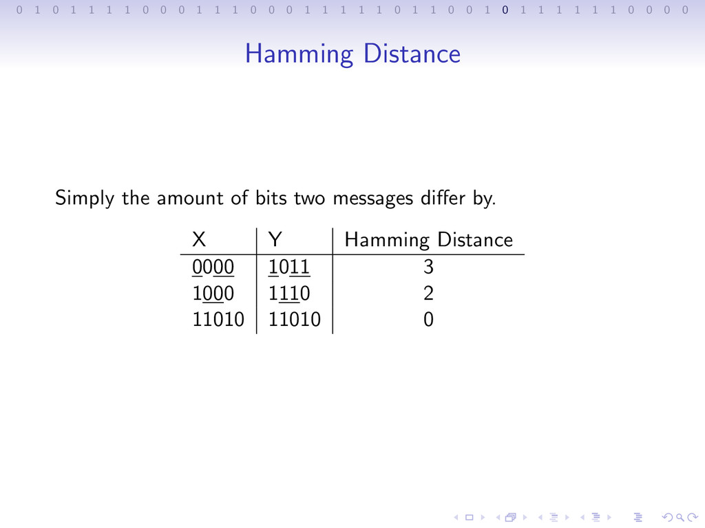
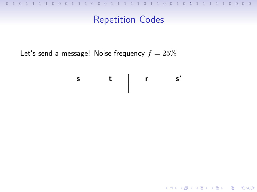
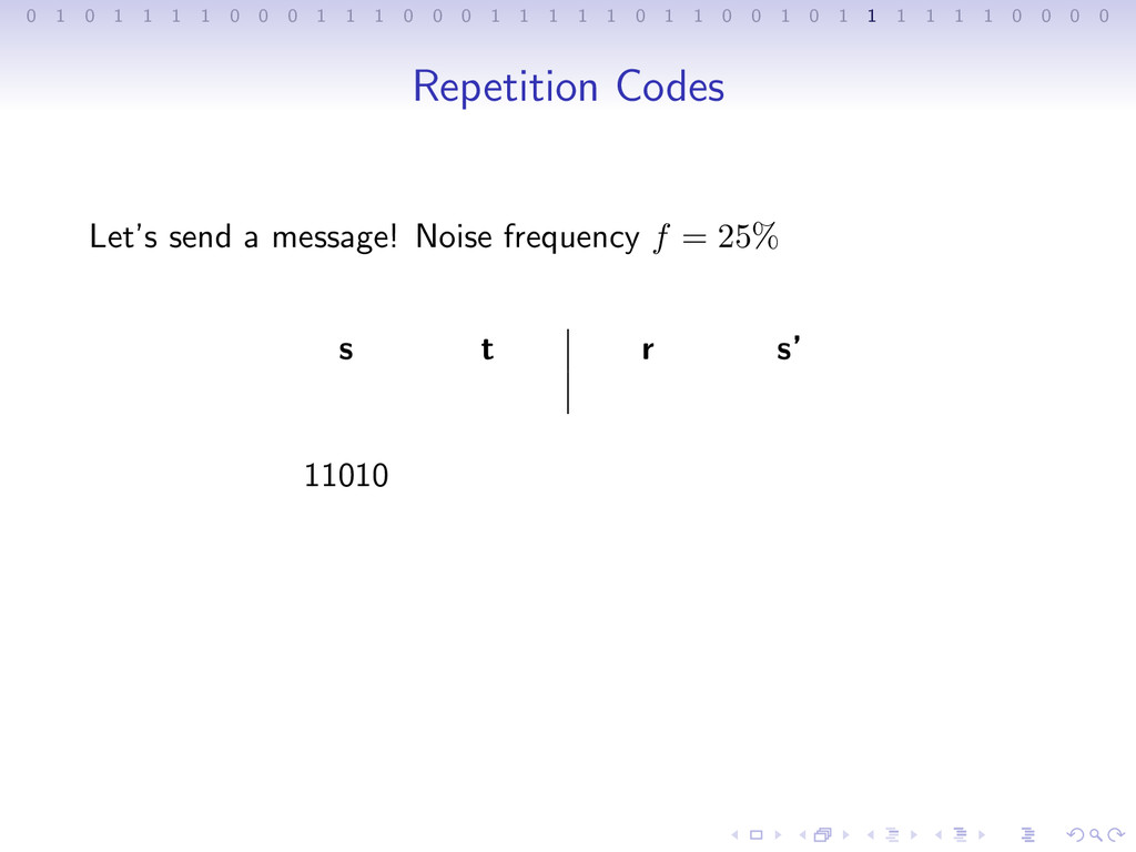
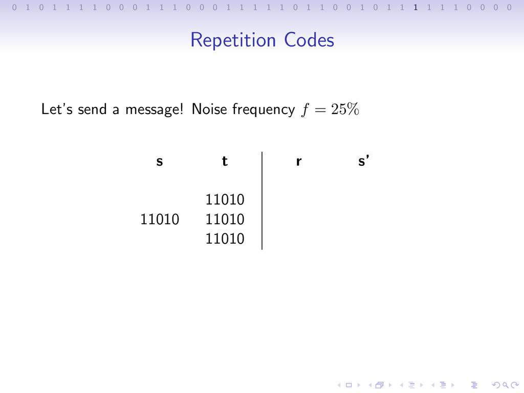
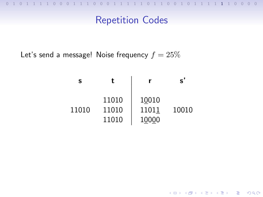
34. 0 1 0 1 1 1 1 0 0 0 1 1 1 0 0 0 1 1 1 1 1 0 1 1 0 0 1 0 1 1 1 1 1 1 0 0 0 0 Repetition Codes Let’s send a message! Noise frequency f = 25% s t r s’ 11010 11010 11010 11010 10010 11011 10000 10010 Hamming distance from s to s’ = 1. Error of 20%. How much, in general, do we reduce the error by?
35. 0 1 0 1 1 1 1 0 0 0 1 1 1 0 0 0 1 1 1 1 1 0 1 1 0 0 1 0 1 1 1 1 1 1 0 0 0 0 Repetition Codes Error Correction in General case:
36. 0 1 0 1 1 1 1 0 0 0 1 1 1 0 0 0 1 1 1 1 1 0 1 1 0 0 1 0 1 1 1 1 1 1 0 0 0 0 Repetition Codes Error Correction in General case: P(errorRN ) = N n=N+1 2 N n fn(1 − f)N−n This is the sum of Binomial probabilities of getting more than half the bits flipped.
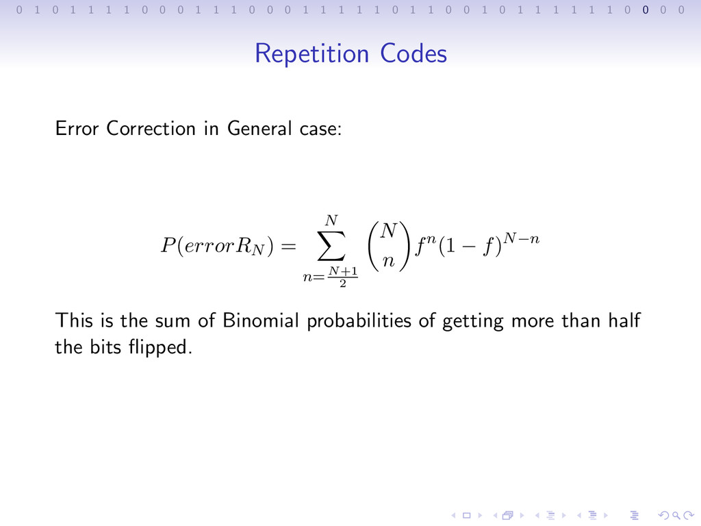
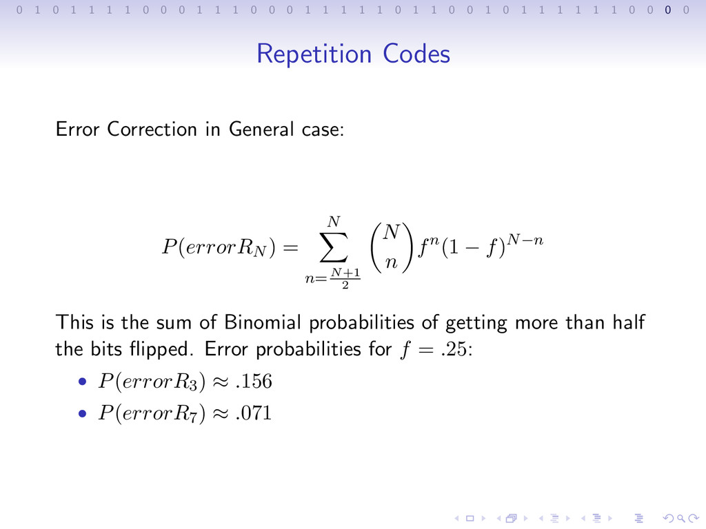
37. 0 1 0 1 1 1 1 0 0 0 1 1 1 0 0 0 1 1 1 1 1 0 1 1 0 0 1 0 1 1 1 1 1 1 0 0 0 0 Repetition Codes Error Correction in General case: P(errorRN ) = N n=N+1 2 N n fn(1 − f)N−n This is the sum of Binomial probabilities of getting more than half the bits flipped. Error probabilities for f = .25: • P(errorR3) ≈ .156 • P(errorR7) ≈ .071
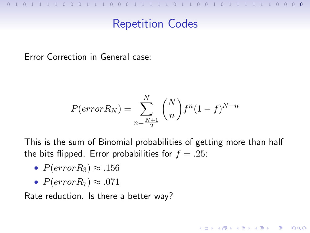
38. 0 1 0 1 1 1 1 0 0 0 1 1 1 0 0 0 1 1 1 1 1 0 1 1 0 0 1 0 1 1 1 1 1 1 0 0 0 0 Repetition Codes Error Correction in General case: P(errorRN ) = N n=N+1 2 N n fn(1 − f)N−n This is the sum of Binomial probabilities of getting more than half the bits flipped. Error probabilities for f = .25: • P(errorR3) ≈ .156 • P(errorR7) ≈ .071 Rate reduction. Is there a better way?
39. 0 1 0 1 1 1 1 0 0 0 1 1 1 0 0 0 1 1 1 1 1 0 1 1 0 0 1 0 1 1 1 1 1 1 0 0 0 0 Joint Entropy and Mutual Information For random variables X = {x1, ..xn} and Y = {y1, ..., ym}:
40. 0 1 0 1 1 1 1 0 0 0 1 1 1 0 0 0 1 1 1 1 1 0 1 1 0 0 1 0 1 1 1 1 1 1 0 0 0 0 Joint Entropy and Mutual Information For random variables X = {x1, ..xn} and Y = {y1, ..., ym}: • Joint Entropy – H(X, Y )
41. 0 1 0 1 1 1 1 0 0 0 1 1 1 0 0 0 1 1 1 1 1 0 1 1 0 0 1 0 1 1 1 1 1 1 0 0 0 0 Joint Entropy and Mutual Information For random variables X = {x1, ..xn} and Y = {y1, ..., ym}: • Joint Entropy – H(X, Y ) = n i=1 m j=1 H(X = xiandY = yj)
42. 0 1 0 1 1 1 1 0 0 0 1 1 1 0 0 0 1 1 1 1 1 0 1 1 0 0 1 0 1 1 1 1 1 1 0 0 0 0 Joint Entropy and Mutual Information For random variables X = {x1, ..xn} and Y = {y1, ..., ym}: • Joint Entropy – H(X, Y ) = n i=1 m j=1 H(X = xiandY = yj) • Mutual Information – I(X : Y )
43. 0 1 0 1 1 1 1 0 0 0 1 1 1 0 0 0 1 1 1 1 1 0 1 1 0 0 1 0 1 1 1 1 1 1 0 0 0 0 Joint Entropy and Mutual Information For random variables X = {x1, ..xn} and Y = {y1, ..., ym}: • Joint Entropy – H(X, Y ) = n i=1 m j=1 H(X = xiandY = yj) • Mutual Information – I(X : Y ) = H(X) + H(Y ) − H(X, Y )
44. 0 1 0 1 1 1 1 0 0 0 1 1 1 0 0 0 1 1 1 1 1 0 1 1 0 0 1 0 1 1 1 1 1 1 0 0 0 0 −0log0? lim x→0+ −xlog2(x) L’Hˆ opital’s Rule If: 1. limx→c f(x) = limx→c = 0 or ±∞ 2. limx→c f (x) g (x) exists 3. g (x) = 0 Then: lim x→c f(x) g(x) = lim x→c f (x) g (x)
45. 0 1 0 1 1 1 1 0 0 0 1 1 1 0 0 0 1 1 1 1 1 0 1 1 0 0 1 0 1 1 1 1 1 1 0 0 0 0 −0log0? lim x→0+ −xlog2(x) L’Hˆ opital’s Rule If: 1. limx→c f(x) = limx→c = 0 or ±∞ 2. limx→c f (x) g (x) exists 3. g (x) = 0 Then: lim x→c f(x) g(x) = lim x→c f (x) g (x) • f(x) = log2(x) → f (x) = 1 x • g(x) = −1 x → g (x) = 1 x2
46. 0 1 0 1 1 1 1 0 0 0 1 1 1 0 0 0 1 1 1 1 1 0 1 1 0 0 1 0 1 1 1 1 1 1 0 0 0 0 −0log0? lim x→0+ −xlog2(x) L’Hˆ opital’s Rule If: 1. limx→c f(x) = limx→c = 0 or ±∞ 2. limx→c f (x) g (x) exists 3. g (x) = 0 Then: lim x→c f(x) g(x) = lim x→c f (x) g (x) • f(x) = log2(x) → f (x) = 1 x • g(x) = −1 x → g (x) = 1 x2 • limx→0+ f(x) g(x) = limx→0+ f (x) g (x) = limx→0+ x2 x = limx→c x = 0
47. 0 1 0 1 1 1 1 0 0 0 1 1 1 0 0 0 1 1 1 1 1 0 1 1 0 0 1 0 1 1 1 1 1 1 0 0 0 0 Example Take two coins, one fair, one two-headed. Choose one randomly (X) and flip it twice. Random variable Y corresponds to the number of heads. X = {0, 1} (fair, unfair), Y = {0, 1, 2} (1 head, 2 heads, 3 heads)
48. 0 1 0 1 1 1 1 0 0 0 1 1 1 0 0 0 1 1 1 1 1 0 1 1 0 0 1 0 1 1 1 1 1 1 0 0 0 0 Example Take two coins, one fair, one two-headed. Choose one randomly (X) and flip it twice. Random variable Y corresponds to the number of heads. X = {0, 1} (fair, unfair), Y = {0, 1, 2} (1 head, 2 heads, 3 heads) X Unfair X=0 H H F=2 H F=2 H H F=2 H F=2 Fair X=1 H H F=2 T F=1 T H F=1 T F=0
49. 0 1 0 1 1 1 1 0 0 0 1 1 1 0 0 0 1 1 1 1 1 0 1 1 0 0 1 0 1 1 1 1 1 1 0 0 0 0 Example Take two coins, one fair, one two-headed. Choose one randomly (X) and flip it twice. Random variable Y corresponds to the number of heads. X = {0, 1} (fair, unfair), Y = {0, 1, 2} (1 head, 2 heads, 3 heads) X Unfair X=0 H H F=2 H F=2 H H F=2 H F=2 Fair X=1 H H F=2 T F=1 T H F=1 T F=0 H(X) H(Y )
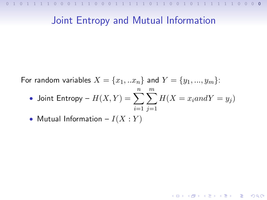
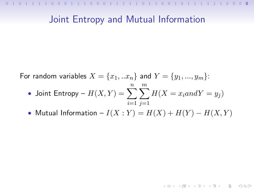
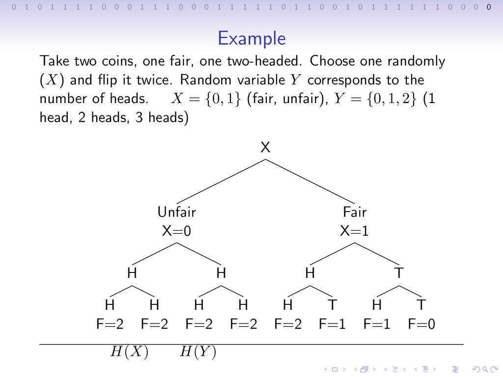
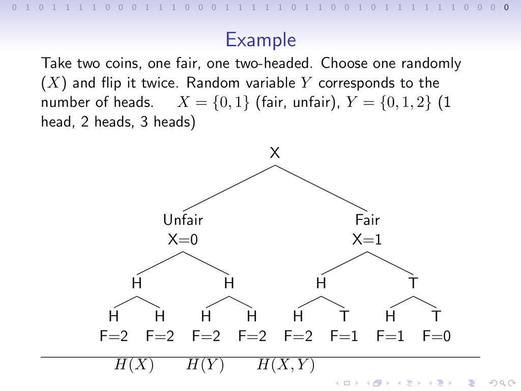
50. 0 1 0 1 1 1 1 0 0 0 1 1 1 0 0 0 1 1 1 1 1 0 1 1 0 0 1 0 1 1 1 1 1 1 0 0 0 0 Example Take two coins, one fair, one two-headed. Choose one randomly (X) and flip it twice. Random variable Y corresponds to the number of heads. X = {0, 1} (fair, unfair), Y = {0, 1, 2} (1 head, 2 heads, 3 heads) X Unfair X=0 H H F=2 H F=2 H H F=2 H F=2 Fair X=1 H H F=2 T F=1 T H F=1 T F=0 H(X) H(Y ) H(X, Y )
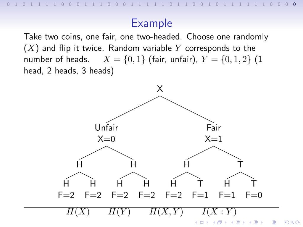
51. 0 1 0 1 1 1 1 0 0 0 1 1 1 0 0 0 1 1 1 1 1 0 1 1 0 0 1 0 1 1 1 1 1 1 0 0 0 0 Example Take two coins, one fair, one two-headed. Choose one randomly (X) and flip it twice. Random variable Y corresponds to the number of heads. X = {0, 1} (fair, unfair), Y = {0, 1, 2} (1 head, 2 heads, 3 heads) X Unfair X=0 H H F=2 H F=2 H H F=2 H F=2 Fair X=1 H H F=2 T F=1 T H F=1 T F=0 H(X) H(Y ) H(X, Y ) I(X : Y )
52. 0 1 0 1 1 1 1 0 0 0 1 1 1 0 0 0 1 1 1 1 1 0 1 1 0 0 1 0 1 1 1 1 1 1 0 0 0 0 As Related to Sets
53. 0 1 0 1 1 1 1 0 0 0 1 1 1 0 0 0 1 1 1 1 1 0 1 1 0 0 1 0 1 1 1 1 1 1 0 0 0 0 More Definitions Assuming channel Λ is a discrete, memoryless, binary symmetric channel (BSC) with error parameter f
54. 0 1 0 1 1 1 1 0 0 0 1 1 1 0 0 0 1 1 1 1 1 0 1 1 0 0 1 0 1 1 1 1 1 1 0 0 0 0 More Definitions Assuming channel Λ is a discrete, memoryless, binary symmetric channel (BSC) with error parameter f • Discrete – Messages can be divided into separate symbols. Furthermore, X and Y have finite target spaces.
55. 0 1 0 1 1 1 1 0 0 0 1 1 1 0 0 0 1 1 1 1 1 0 1 1 0 0 1 0 1 1 1 1 1 1 0 0 0 0 More Definitions Assuming channel Λ is a discrete, memoryless, binary symmetric channel (BSC) with error parameter f • Discrete – Messages can be divided into separate symbols. Furthermore, X and Y have finite target spaces. • Memoryless – Probabilities are independent and don’t change.
56. 0 1 0 1 1 1 1 0 0 0 1 1 1 0 0 0 1 1 1 1 1 0 1 1 0 0 1 0 1 1 1 1 1 1 0 0 0 0 More Definitions Assuming channel Λ is a discrete, memoryless, binary symmetric channel (BSC) with error parameter f • Discrete – Messages can be divided into separate symbols. Furthermore, X and Y have finite target spaces. • Memoryless – Probabilities are independent and don’t change. • Binary Symmetric Channel – Channel with binary input and binary output and error parameter f < .5
57. 0 1 0 1 1 1 1 0 0 0 1 1 1 0 0 0 1 1 1 1 1 0 1 1 0 0 1 0 1 1 1 1 1 1 0 0 0 0 More Definitions Assuming channel Λ is a discrete, memoryless, binary symmetric channel (BSC) with error parameter f • Discrete – Messages can be divided into separate symbols. Furthermore, X and Y have finite target spaces. • Memoryless – Probabilities are independent and don’t change. • Binary Symmetric Channel – Channel with binary input and binary output and error parameter f < .5 • Redundancy – Extra information added to a message to reduce error.
58. 0 1 0 1 1 1 1 0 0 0 1 1 1 0 0 0 1 1 1 1 1 0 1 1 0 0 1 0 1 1 1 1 1 1 0 0 0 0 More Definitions Assuming channel Λ is a discrete, memoryless, binary symmetric channel (BSC) with error parameter f • Discrete – Messages can be divided into separate symbols. Furthermore, X and Y have finite target spaces. • Memoryless – Probabilities are independent and don’t change. • Binary Symmetric Channel – Channel with binary input and binary output and error parameter f < .5 • Redundancy – Extra information added to a message to reduce error. • Capacity – Maximum concentration of information for a given channel. Γ = maxP(X) I(X : Y )
59. 0 1 0 1 1 1 1 0 0 0 1 1 1 0 0 0 1 1 1 1 1 0 1 1 0 0 1 0 1 1 1 1 1 1 0 0 0 0 More Definitions Assuming channel Λ is a discrete, memoryless, binary symmetric channel (BSC) with error parameter f • Discrete – Messages can be divided into separate symbols. Furthermore, X and Y have finite target spaces. • Memoryless – Probabilities are independent and don’t change. • Binary Symmetric Channel – Channel with binary input and binary output and error parameter f < .5 • Redundancy – Extra information added to a message to reduce error. • Capacity – Maximum concentration of information for a given channel. Γ = maxP(X) I(X : Y ) Simplifies to Γ = 1 − H(f)
60. 0 1 0 1 1 1 1 0 0 0 1 1 1 0 0 0 1 1 1 1 1 0 1 1 0 0 1 0 1 1 1 1 1 1 0 0 0 0 Fundamental Theorem Goal: to minimize error probability, while also minimizing redundancy (and thereby maximize rate).
61. 0 1 0 1 1 1 1 0 0 0 1 1 1 0 0 0 1 1 1 1 1 0 1 1 0 0 1 0 1 1 1 1 1 1 0 0 0 0 Fundamental Theorem Goal: to minimize error probability, while also minimizing redundancy (and thereby maximize rate). Let Λ be a BSC with parameter f < 1/2 and resulting capacity Γ = 1 − H(f). Let R be any information rate with R < Γ. Let > 0 be an arbitrarily small positive quantity. Then, there exists a code C of length N and a rate ≥ R and a decoding algorithm such that the maximum probability of error is ≤ .
62. 0 1 0 1 1 1 1 0 0 0 1 1 1 0 0 0 1 1 1 1 1 0 1 1 0 0 1 0 1 1 1 1 1 1 0 0 0 0 Fundamental Theorem Goal: to minimize error probability, while also minimizing redundancy (and thereby maximize rate). Let Λ be a BSC with parameter f < 1/2 and resulting capacity Γ = 1 − H(f). Let R be any information rate with R < Γ. Let > 0 be an arbitrarily small positive quantity. Then, there exists a code C of length N and a rate ≥ R and a decoding algorithm such that the maximum probability of error is ≤ . • Baby analogy
63. 0 1 0 1 1 1 1 0 0 0 1 1 1 0 0 0 1 1 1 1 1 0 1 1 0 0 1 0 1 1 1 1 1 1 0 0 0 0 Fundamental Theorem Goal: to minimize error probability, while also minimizing redundancy (and thereby maximize rate). Let Λ be a BSC with parameter f < 1/2 and resulting capacity Γ = 1 − H(f). Let R be any information rate with R < Γ. Let > 0 be an arbitrarily small positive quantity. Then, there exists a code C of length N and a rate ≥ R and a decoding algorithm such that the maximum probability of error is ≤ . • Baby analogy • R > Γ
64. 0 1 0 1 1 1 1 0 0 0 1 1 1 0 0 0 1 1 1 1 1 0 1 1 0 0 1 0 1 1 1 1 1 1 0 0 0 0 Hamming Code and Parity • Richard Hamming
65. 0 1 0 1 1 1 1 0 0 0 1 1 1 0 0 0 1 1 1 1 1 0 1 1 0 0 1 0 1 1 1 1 1 1 0 0 0 0 Hamming Code and Parity • Richard Hamming – (7,4)Hamming Code
66. 0 1 0 1 1 1 1 0 0 0 1 1 1 0 0 0 1 1 1 1 1 0 1 1 0 0 1 0 1 1 1 1 1 1 0 0 0 0 Hamming Code and Parity • Richard Hamming – (7,4)Hamming Code • SECDED
67. 0 1 0 1 1 1 1 0 0 0 1 1 1 0 0 0 1 1 1 1 1 0 1 1 0 0 1 0 1 1 1 1 1 1 0 0 0 0 Hamming Code and Parity • Richard Hamming – (7,4)Hamming Code • SECDED • General – (n,k)Hamming Codes: n message length, r parity bits, and k data bits, where n = 2r − 1, k = 2r − r − 1 = n − r, and r ≥ 2.
68. 0 1 0 1 1 1 1 0 0 0 1 1 1 0 0 0 1 1 1 1 1 0 1 1 0 0 1 0 1 1 1 1 1 1 0 0 0 0 Hamming Code and Parity • Richard Hamming – (7,4)Hamming Code • SECDED • General – (n,k)Hamming Codes: n message length, r parity bits, and k data bits, where n = 2r − 1, k = 2r − r − 1 = n − r, and r ≥ 2. r n k rate = k n 2 3 1 .3333 3 7 4 .5714 4 15 11 .7333 5 31 26 .8387 . . . . . . 10 1023 1013 .9902 . . . . . . 16 65535 65519 .9996
69. 0 1 0 1 1 1 1 0 0 0 1 1 1 0 0 0 1 1 1 1 1 0 1 1 0 0 1 0 1 1 1 1 1 1 0 0 0 0 Application 1 – QR Codes • Use Reed-Solomon error correction with 8 bit codewords. • Block errors Level Approx. codewords restored L 7% M 15% Q 32% H 30%
70. 0 1 0 1 1 1 1 0 0 0 1 1 1 0 0 0 1 1 1 1 1 0 1 1 0 0 1 0 1 1 1 1 1 1 0 0 0 0
71. 0 1 0 1 1 1 1 0 0 0 1 1 1 0 0 0 1 1 1 1 1 0 1 1 0 0 1 0 1 1 1 1 1 1 0 0 0 0 Application 2 – DNA • DNA as code: 4 base pairs: (A, C, G, T) • Quaternary system - easy to make Binary
72. 0 1 0 1 1 1 1 0 0 0 1 1 1 0 0 0 1 1 1 1 1 0 1 1 0 0 1 0 1 1 1 1 1 1 0 0 0 0 Application 2 – DNA • DNA as code: 4 base pairs: (A, C, G, T) • Quaternary system - easy to make Binary • About 3.2 Billion base pairs: 6.4 Billion bits or about 800 Megabytes. Testament?
73. 0 1 0 1 1 1 1 0 0 0 1 1 1 0 0 0 1 1 1 1 1 0 1 1 0 0 1 0 1 1 1 1 1 1 0 0 0 0 Application 2 – DNA • DNA as code: 4 base pairs: (A, C, G, T) • Quaternary system - easy to make Binary • About 3.2 Billion base pairs: 6.4 Billion bits or about 800 Megabytes. Testament? • Competing goals: prokaryotes vs. eukaryotes
74. 0 1 0 1 1 1 1 0 0 0 1 1 1 0 0 0 1 1 1 1 1 0 1 1 0 0 1 0 1 1 1 1 1 1 0 0 0 0 Application 2 – DNA • DNA as code: 4 base pairs: (A, C, G, T) • Quaternary system - easy to make Binary • About 3.2 Billion base pairs: 6.4 Billion bits or about 800 Megabytes. Testament? • Competing goals: prokaryotes vs. eukaryotes • Field of Bioinformatics
75. 0 1 0 1 1 1 1 0 0 0 1 1 1 0 0 0 1 1 1 1 1 0 1 1 0 0 1 0 1 1 1 1 1 1 0 0 0 0 Sources Primary Sources 1. Aiden A. Bruen and Mario A. Forcintino. Cryptography, Information Theory, and Error-Correction John Wiley Sons, 2005. 2. David J. C. MacKay. Information Theory, Inference, and Learning Algorithms Cambridge University Press, 2003. Papers 1. Claude E. Shannon, Warren Weaver. The Mathematical Theory of Communication Univ of Illinois Press, 1949. 2. Thomas A. Kunkel. DNA Replication Fidelity JBC Papers 2004.