Upgrade to Pro — share decks privately, control downloads, hide ads and more …

Machine Learning: The Bare Math Behind Libraries

rauluka7
November 08, 2019

Machine Learning: The Bare Math Behind Libraries

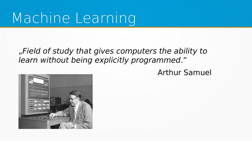
Machine learning is one of the hottest buzzwords in technology today as well as one of the most innovative fields in computer science – yet people use libraries as black boxes without basic knowledge of the field. In this session, we will strip them to bare math, so next time you use a machine learning library, you'll have a deeper understanding of what lies underneath.

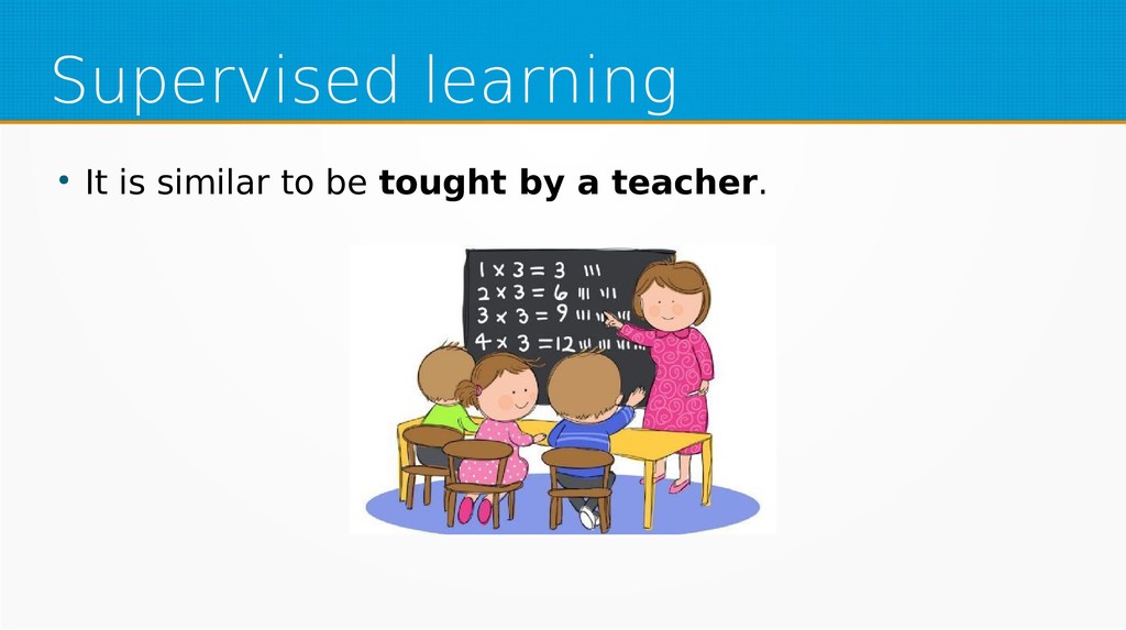
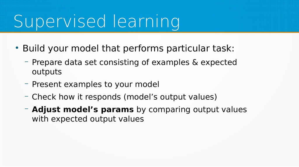
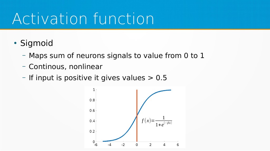
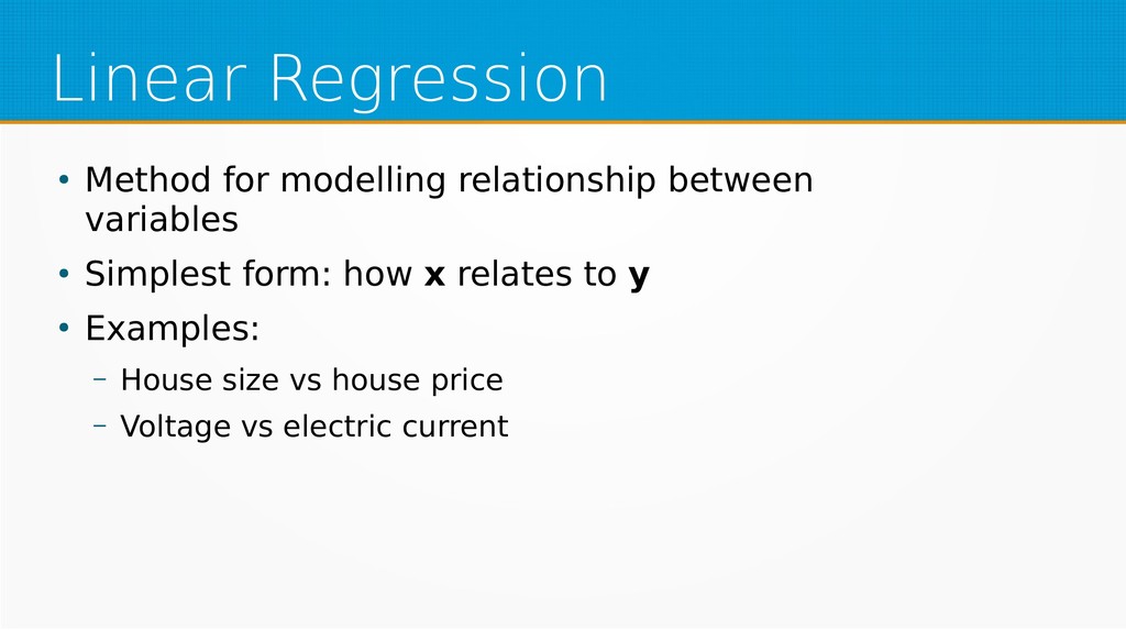
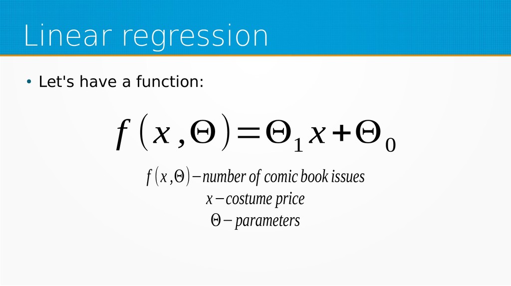
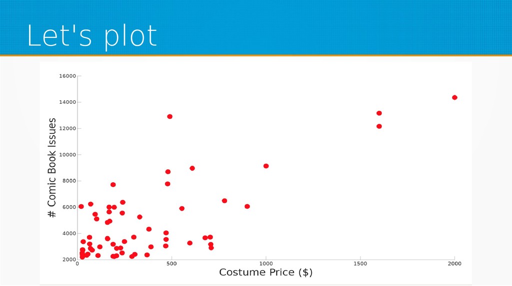
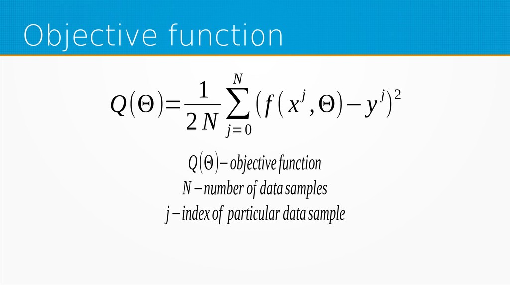
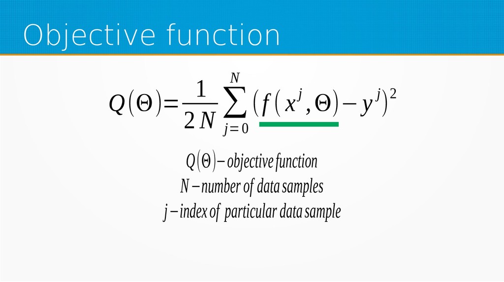
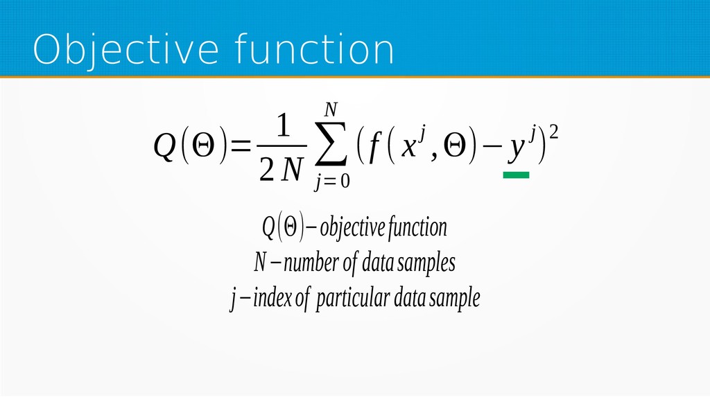
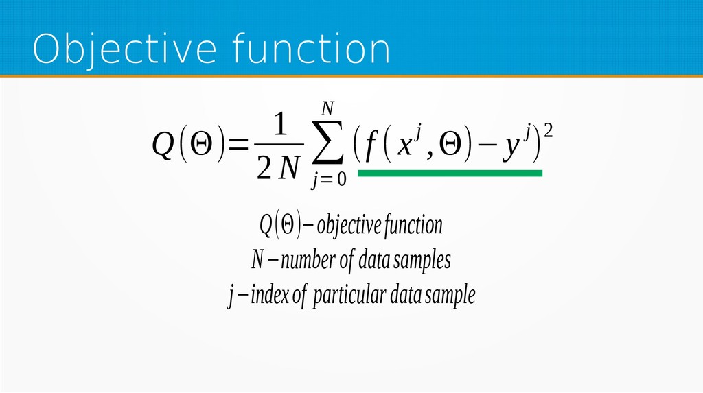
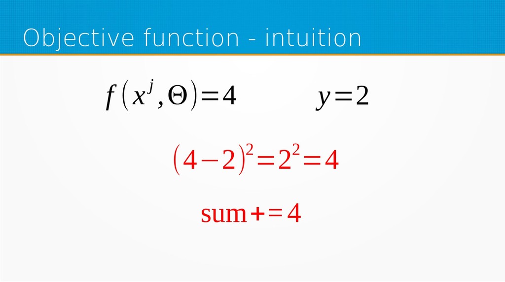
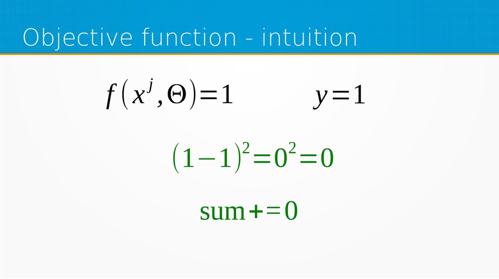
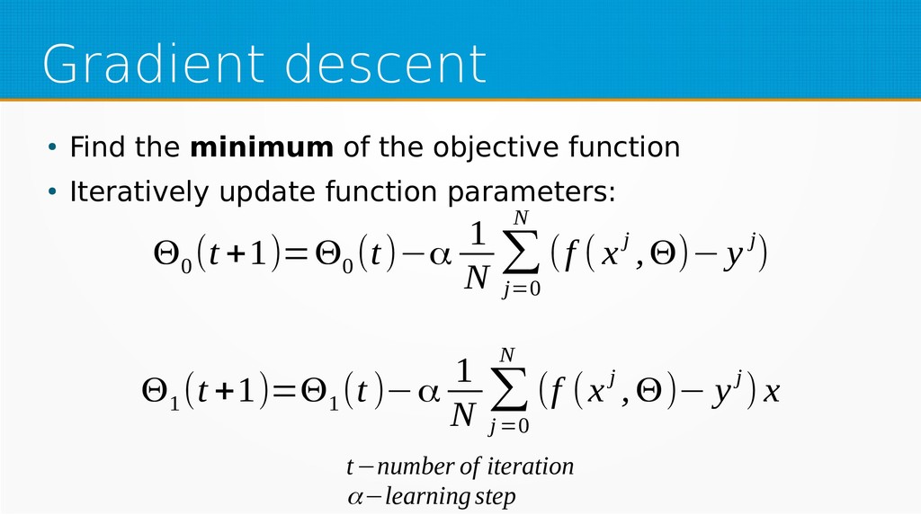
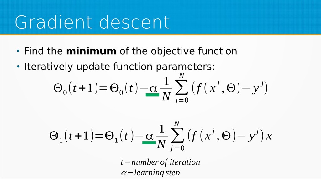
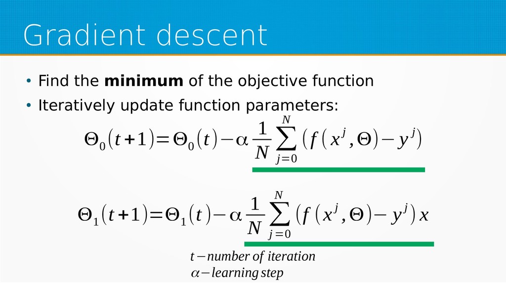
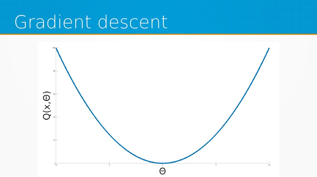
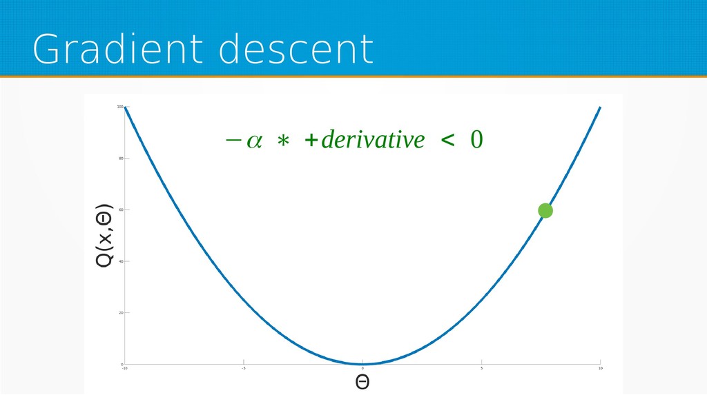
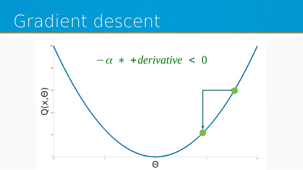
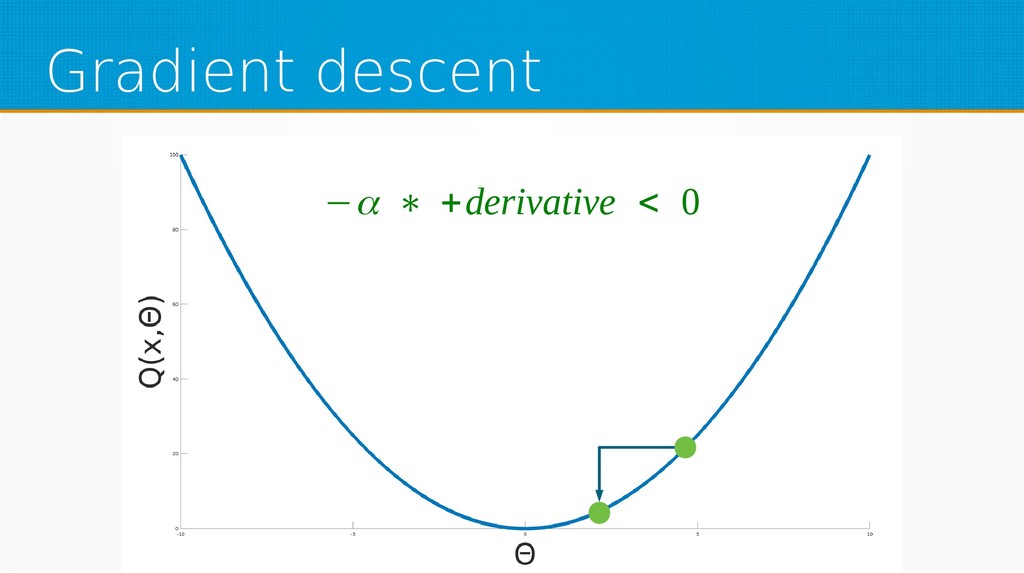
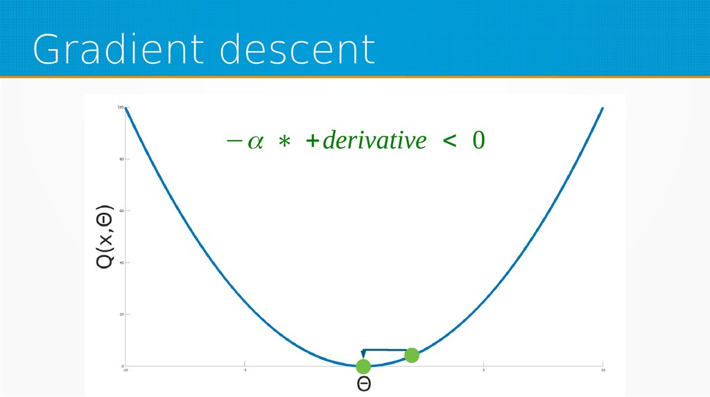
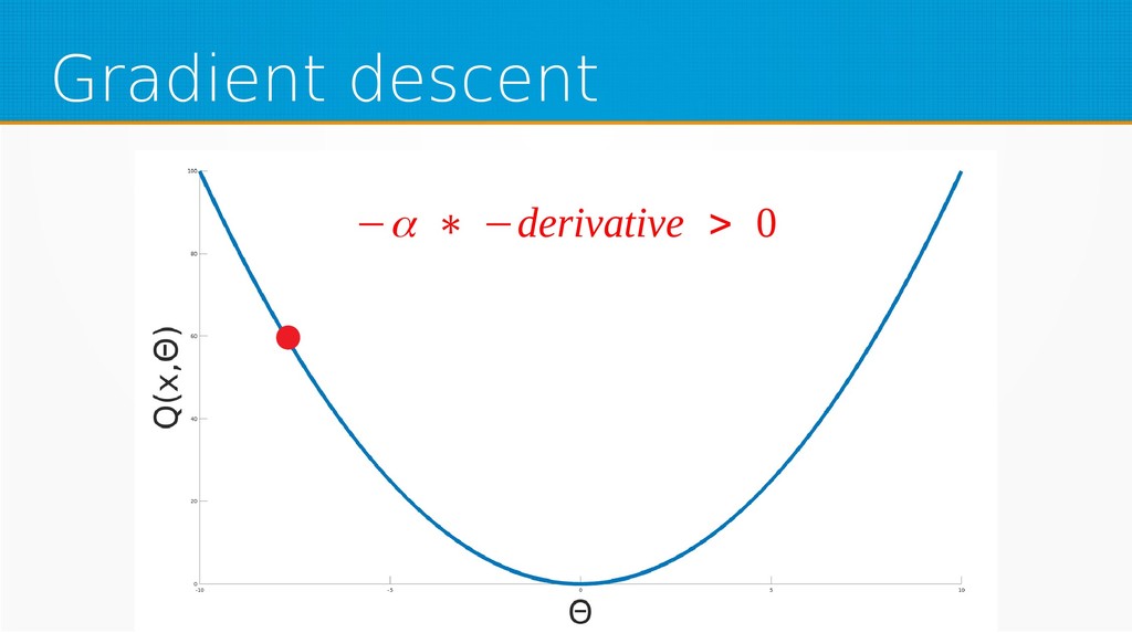
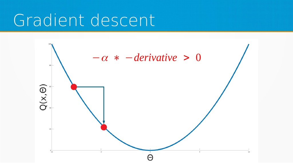
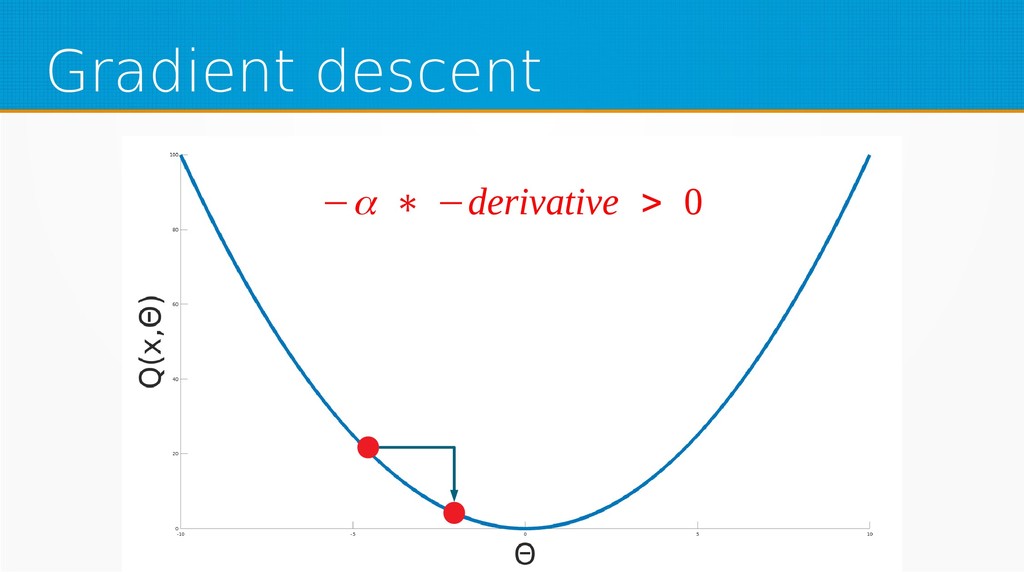
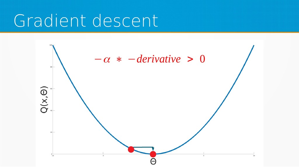
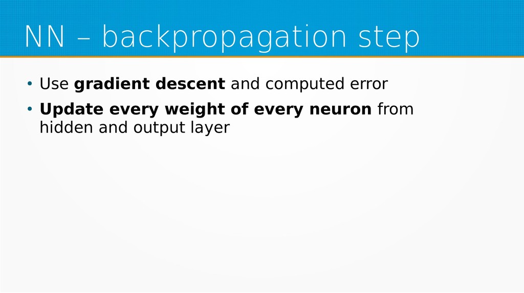
During this session, we will first provide a short history of machine learning and an overview of two basic teaching techniques: supervised and unsupervised learning. We will start by defining what machine learning is and equip you with an intuition of how it works. We will then explain gradient descent algorithm with the use of simple linear regression to give you an even deeper understanding of this learning method.

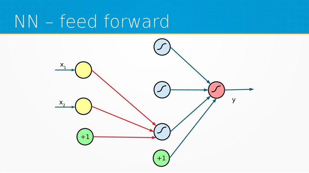
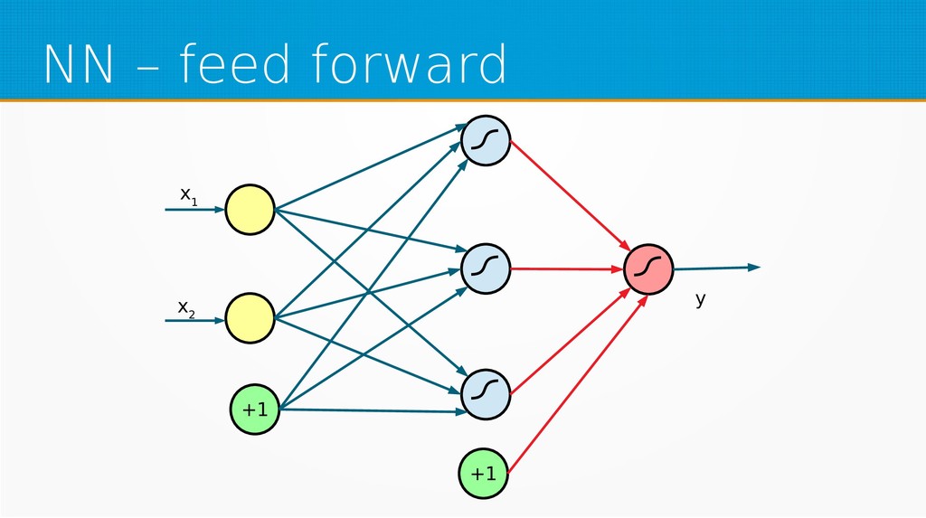
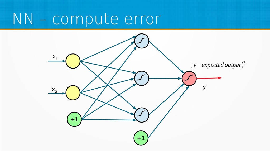
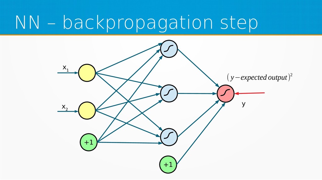
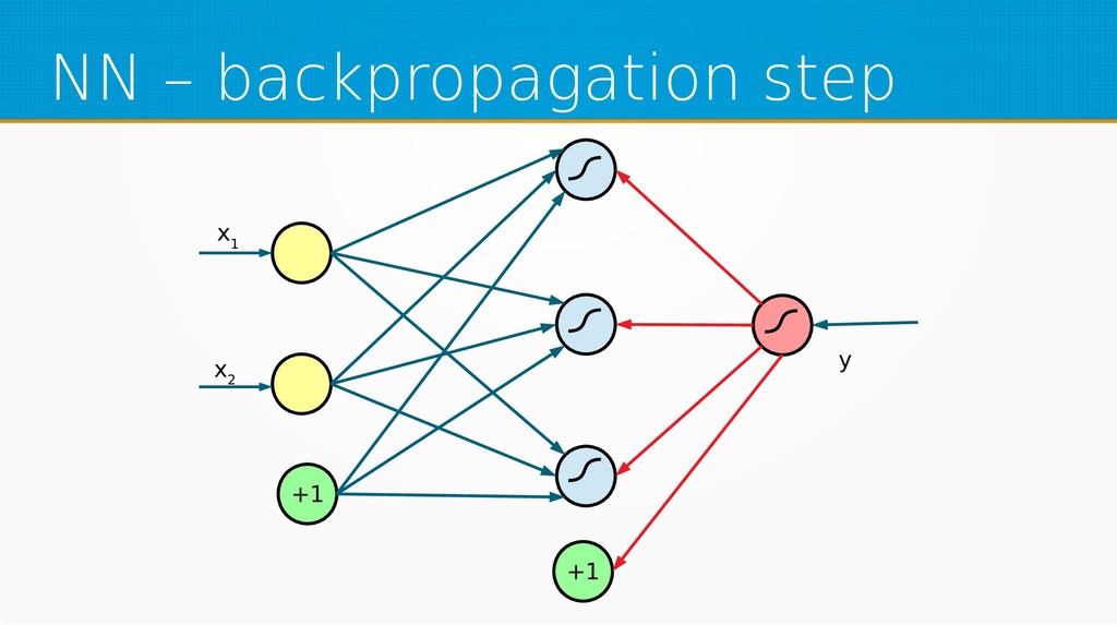
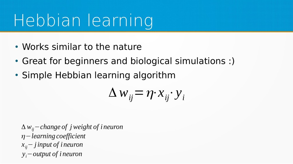
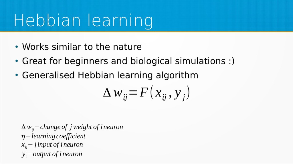
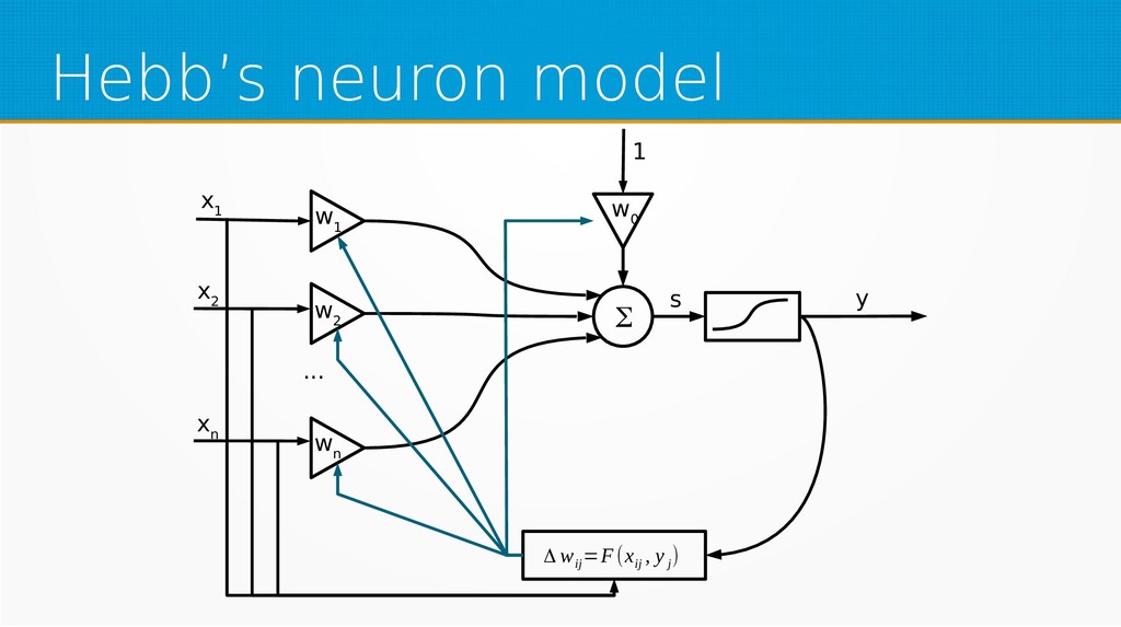
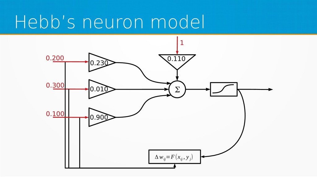
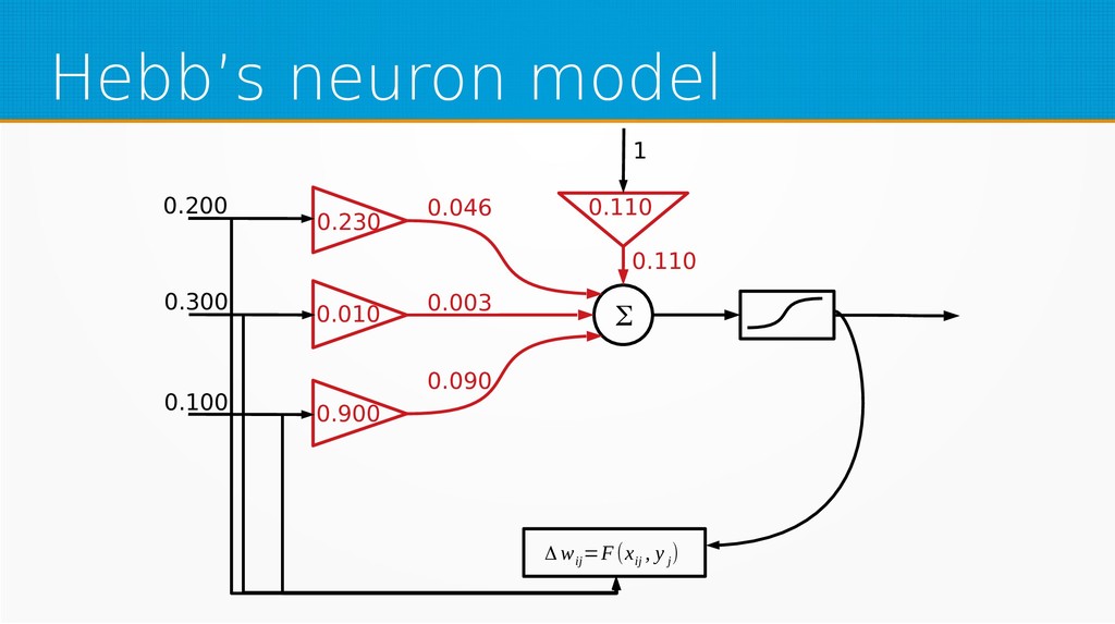
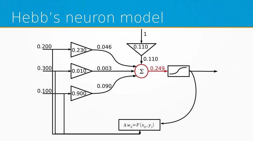
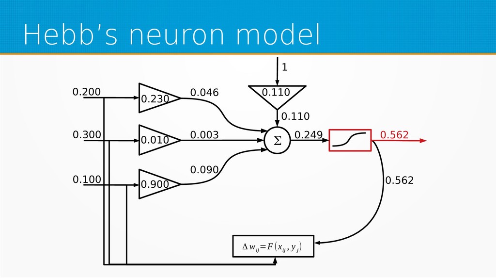
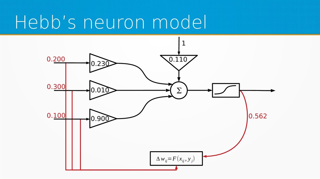
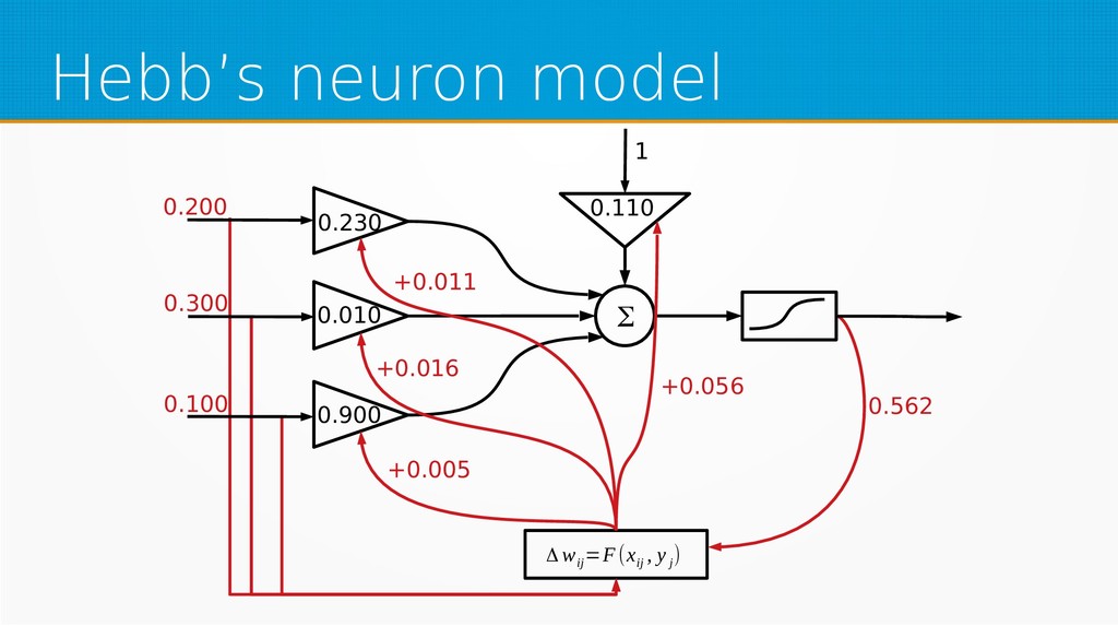
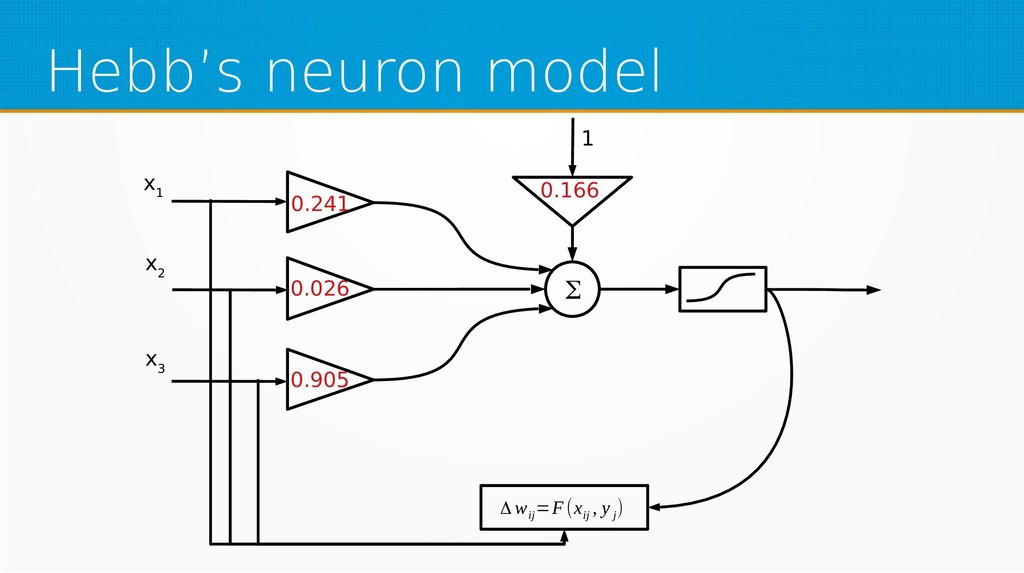
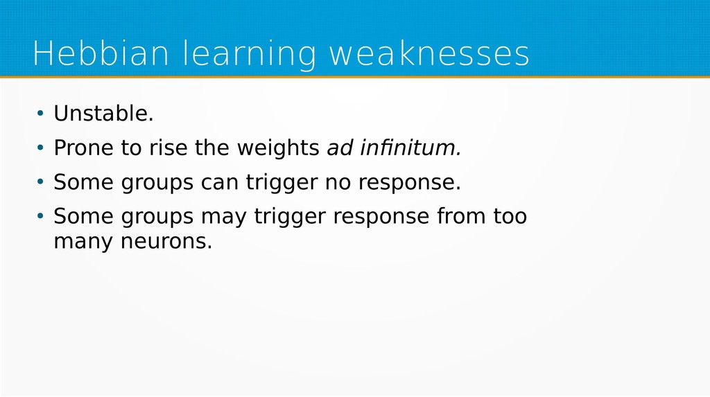
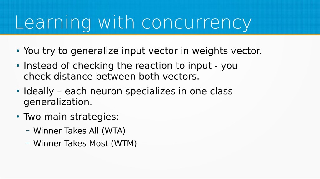
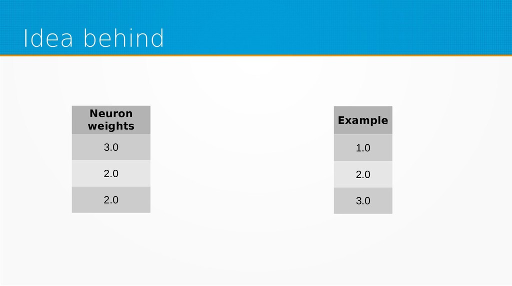
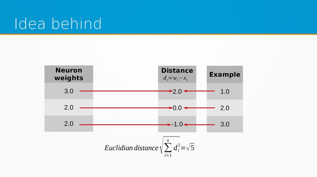
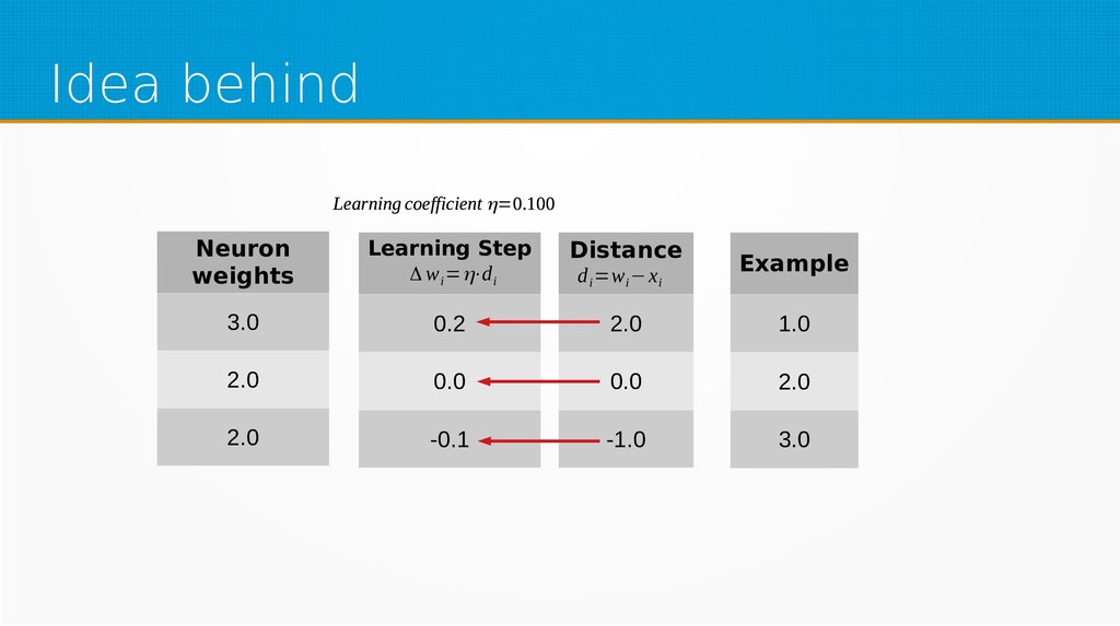
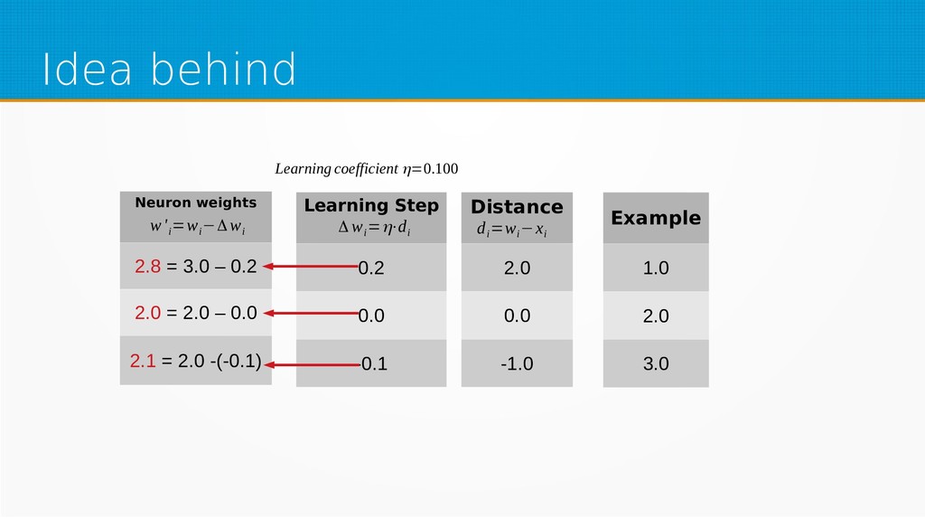
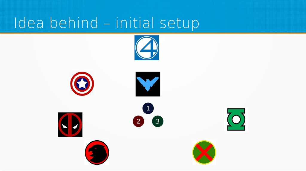
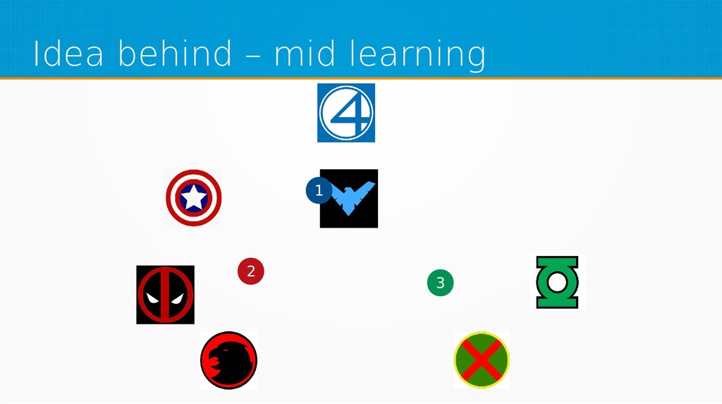
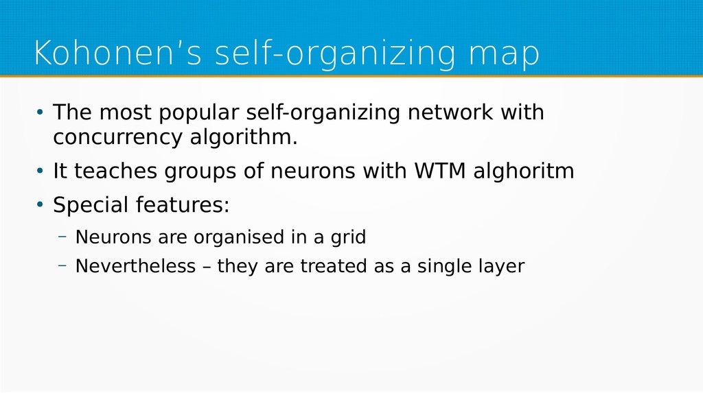
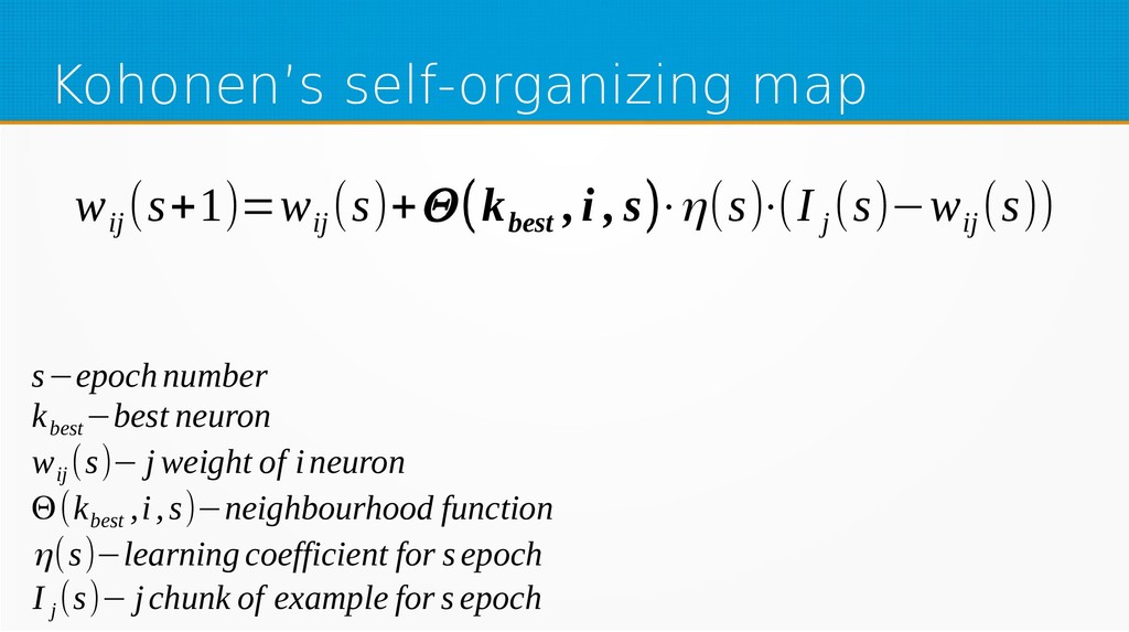
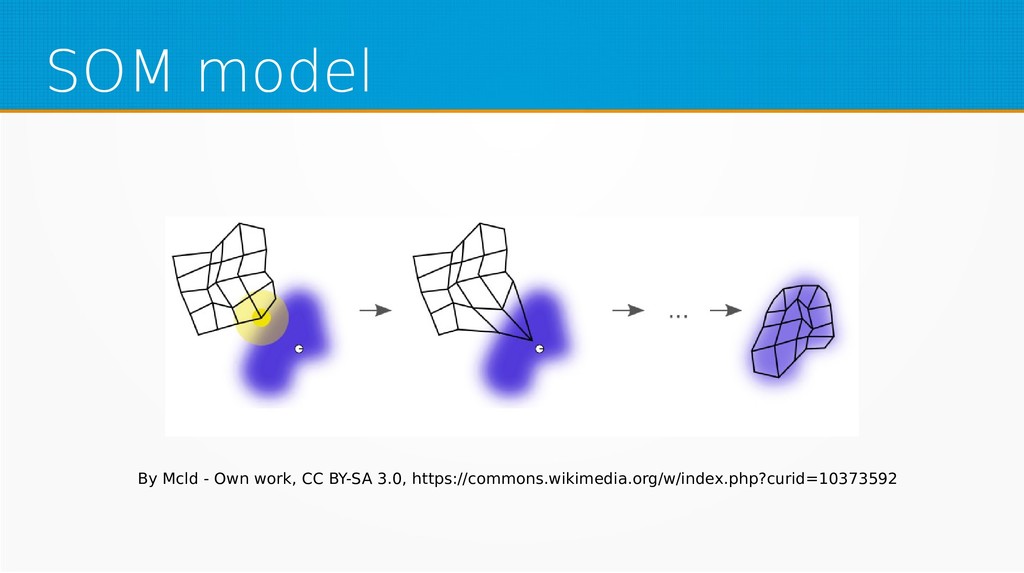
Then we will project it to supervised neural networks training. Within unsupervised learning, you will become familiar with Hebb’s learning and learning with concurrency (winner takes all and winner takes most algorithms).

We will use Octave for examples in this session; however, you can use your favorite technology to implement presented ideas. Our aim is to show the mathematical basics of neural networks for those who want to start using machine learning in their day-to-day work or use it already but find it difficult to understand the underlying processes.

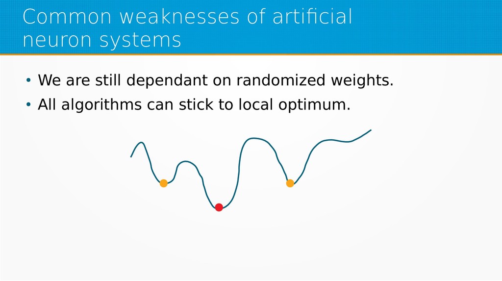
After viewing our presentation, you should find it easier to select parameters for your networks and feel more confident in your selection of network type, as well as be encouraged to dive into more complex and powerful deep learning methods.

rauluka7

November 08, 2019
Tweet

More Decks by rauluka7

Other Decks in Programming

Transcript

  1. @YourTwitterHandle #Devoxx #YourTag Machine Learning: The Bare Math Behind Libraries

    Machine Learning: The Bare Math Behind Libraries Piotr Czajka & Łukasz Gebel TomTom @medwith @rauluka7
  2. Machine Learning „Field of study that gives computers the ability

    to learn without being explicitly programmed.” Arthur Samuel
  3. Machine Learning „I consider every method that needs training as

    intelligent or machine learning method.” Our Lecturer
  4. Supervised learning • Build your model that performs particular task:

    – Prepare data set consisting of examples & expected outputs
  5. Supervised learning • Build your model that performs particular task:

    – Prepare data set consisting of examples & expected outputs – Present examples to your model
  6. Supervised learning • Build your model that performs particular task:

    – Prepare data set consisting of examples & expected outputs – Present examples to your model – Check how it responds (model’s output values)
  7. Supervised learning • Build your model that performs particular task:

    – Prepare data set consisting of examples & expected outputs – Present examples to your model – Check how it responds (model’s output values) – Adjust model’s params by comparing output values with expected output values
  8. Neural Networks • Inspired by biological brain mechanisms • Many

    applications: – Computer vision – Speech recognition – Compression
  9. Artificial Neuron • Inputs (x 1, … , x n

    ) are features of single example • Multiply each input by weight, sum it and put the sum as an argument of activation function w 1 w 2 w n w 0 Σ x 1 x 2 x n ... s y
  10. Activation function • Sigmoid – Maps sum of neurons signals

    to value from 0 to 1 – Continous, nonlinear – If input is positive it gives values > 0.5 f (x)= 1 1+e(−βx)
  11. Linear Regression • Method for modelling relationship between variables •

    Simplest form: how x relates to y • Examples: – House size vs house price – Voltage vs electric current
  12. Costume price vs number of issues • For given amount

    of money predict in how many comic book issues you’ll appear. Costume price(x) Number of issues (y) 240 6370 480 8697 ... ... 26 2200
  13. Linear regression • Let's have a function: f (x ,Θ)=Θ1

    x+Θ0 f (x,Θ)−number of comicbookissues x−costume price Θ−parameters
  14. Objective function Q(Θ)= 1 2 N ∑ j=0 N (f

    ( xj ,Θ)−y j )2 Q(Θ)−objectivefunction N−numberof datasamples j−indexof particulardatasample
  15. Objective function Q(Θ)= 1 2 N ∑ j=0 N (f

    ( xj ,Θ)−y j )2 Q(Θ)−objectivefunction N−numberof datasamples j−indexof particulardatasample
  16. Objective function Q(Θ)= 1 2 N ∑ j=0 N (f

    ( xj ,Θ)−y j )2 Q(Θ)−objectivefunction N−numberof datasamples j−indexof particulardatasample
  17. Objective function Q(Θ)= 1 2 N ∑ j=0 N (f

    ( xj ,Θ)−y j )2 Q(Θ)−objectivefunction N−numberof datasamples j−indexof particulardatasample
  18. Gradient descent • Find the minimum of the objective function

    • Iteratively update function parameters: Θ0 (t +1)=Θ0 (t)−α 1 N ∑ j=0 N (f ( xj ,Θ)− y j ) Θ1 (t +1)=Θ1 (t )−α 1 N ∑ j=0 N (f (xj ,Θ)− yj ) x t−number of iteration α−learning step
  19. Gradient descent • Find the minimum of the objective function

    • Iteratively update function parameters: Θ0 (t +1)=Θ0 (t)−α 1 N ∑ j=0 N (f ( xj ,Θ)− y j ) Θ1 (t +1)=Θ1 (t )−α 1 N ∑ j=0 N (f (xj ,Θ)− yj ) x t−number of iteration α−learning step
  20. Gradient descent • Find the minimum of the objective function

    • Iteratively update function parameters: Θ0 (t +1)=Θ0 (t)−α 1 N ∑ j=0 N (f ( xj ,Θ)− y j ) Θ1 (t +1)=Θ1 (t )−α 1 N ∑ j=0 N (f (xj ,Θ)− yj ) x t−number of iteration α−learning step
  21. NN – compute error +1 +1 x 1 x 2

    y ( y−expected output)2
  22. NN – backpropagation step • Use gradient descent and computed

    error • Update every weight of every neuron from hidden and output layer
  23. NN – backpropagation step +1 +1 x 1 x 2

    y ( y−expected output)2
  24. Real life problem • You said it can solve non

    linear problems, let's generate superhero logo using it.
  25. Why would we let them? • Less complex mathematical apparatus

    than in supervised learning. • It is similar to discovering world on your own.
  26. Why would we let them? Used mostly for sorting and

    grouping when: • Sorting key can’t be easily figured out. • Data is very complex and finding the key is not trivial.
  27. Hebbian learning • Works similar to the nature • Great

    for beginners and biological simulations :) • Simple Hebbian learning algorithm Δ w ij =η⋅x ij ⋅y i Δ w ij −change of j weight of ineuron η−learningcoefficient x ij − jinput of ineuron y i −output of i neuron
  28. Hebbian learning • Works similar to the nature • Great

    for beginners and biological simulations :) • Generalised Hebbian learning algorithm Δ w ij =F(x ij , y j ) Δ w ij −change of j weight of ineuron η−learningcoefficient x ij − jinput of ineuron y i −output of i neuron
  29. Hebb’s neuron model w 1 w 2 w n w

    0 Δ w ij =F(x ij , y j ) Σ x 1 x 2 x n ... 1 s y
  30. Hebb’s neuron model 0.230 0.010 0.900 0.110 Δ w ij

    =F(x ij , y j ) Σ 0.200 0.300 0.100 1
  31. Hebb’s neuron model 0.230 0.010 0.900 0.110 Δ w ij

    =F(x ij , y j ) Σ 1 0.046 0.003 0.090 0.110 0.200 0.300 0.100
  32. Hebb’s neuron model 0.230 0.010 0.900 0.110 Δ w ij

    =F(x ij , y j ) Σ 1 0.046 0.003 0.090 0.110 0.249 0.200 0.300 0.100
  33. Hebb’s neuron model 0.230 0.010 0.900 0.110 Δ w ij

    =F(x ij , y j ) Σ 1 0.046 0.003 0.090 0.110 0.249 0.562 0.562 0.200 0.300 0.100
  34. Hebb’s neuron model 0.230 0.010 0.900 0.110 Δ w ij

    =F(x ij , y j ) Σ 1 0.562 0.200 0.300 0.100
  35. Hebb’s neuron model 0.230 0.010 0.900 0.110 Δ w ij

    =F(x ij , y j ) Σ 1 0.562 +0.011 +0.016 +0.005 +0.056 0.300 0.100 0.200
  36. Marvel database to the rescue Intelligence Strength Speed Durability Energy

    projection Fighting skills Iron Man 6 6 5 6 6 4 Spiderman 4 4 3 3 1 4 Black Panter 5 3 2 3 3 5 Wolverine 2 4 2 4 1 7 Thor 2 7 7 6 6 4 Dr Strange 4 2 7 2 6 6 Hulk 2 7 3 7 5 4 Cpt. America 3 3 2 3 1 6 Mr Fantastic 6 2 2 5 1 3 Human Torch 2 2 5 2 5 3 Invisible Woman 3 2 3 6 5 3 The Thing 3 6 2 6 1 5 Luke Cage 3 4 2 5 1 4 She Hulk 3 7 3 6 1 4 Ms Marvel 2 6 2 6 1 4 Daredevil 3 3 2 2 4 5
  37. Hebbian learning weaknesses • Unstable. • Prone to rise the

    weights ad infinitum. • Some groups can trigger no response. • Some groups may trigger response from too many neurons.
  38. Learning with concurrency • You try to generalize input vector

    in weights vector. • Instead of checking the reaction to input - you check distance between both vectors. • Ideally – each neuron specializes in one class generalization. • Two main strategies: – Winner Takes All (WTA) – Winner Takes Most (WTM)
  39. Example 1.0 2.0 3.0 Idea behind Distance 2.0 0.0 -1.0

    Neuron weights 3.0 2.0 2.0 d i =w i −x i Euclidiandistance √∑ i=1 n d i 2 =√5
  40. Distance 2.0 0.0 -1.0 Idea behind Neuron weights 3.0 2.0

    2.0 Learning coefficient η=0.100 Learning Step 0.2 0.0 -0.1 Δ w i =η⋅d i Example 1.0 2.0 3.0 d i =w i −x i Learning coefficient η=0.100
  41. Idea behind Distan ce 2.0 0.0 -1.0 Neuron weights 2.8

    = 3.0 – 0.2 2.0 = 2.0 – 0.0 2.1 = 2.0 -(-0.1) Exam ple 1.0 2.0 3.0 d i =w i −x i Learning coefficient η=0.100 Learning Step 0.2 0.0 -0.1 w' i =w i −Δw i Δ w i =η⋅d i Example 1.0 2.0 3.0 Learning Step 0.2 0.0 -0.1 Δ w i =η⋅d i Distance 2.0 0.0 -1.0 d i =w i −x i
  42. Learning with concurrency • Gives more diverse groups. • Less

    prone to clustering (than Hebb’s). • Searches wider spectrum of answers. • First step to more complex networks.
  43. Learning with concurency - weaknesses • WTA – works best

    if teaching examples are evenly distributed in solution space. • WTM – works best if weights’ vectors are evenly distributed in solution space. • Still can stick to local optimum.
  44. Kohonen’s self-organizing map • The most popular self-organizing network with

    concurrency algorithm. • It teaches groups of neurons with WTM alghoritm • Special features: – Neurons are organised in a grid – Nevertheless – they are treated as a single layer
  45. Kohonen’s self-organizing map w ij (s+1)=w ij (s)+Θ(k best ,i

    , s)⋅η(s)⋅(I j (s)−w ij (s)) s−epochnumber k best −best neuron w ij (s)− j weight of ineuron Θ(k best ,i,s)−neighbourhood function η(s)−learning coefficient for sepoch I j (s)− jchunk of example for s epoch
  46. SOM model By Mcld - Own work, CC BY-SA 3.0,

    https://commons.wikimedia.org/w/index.php?curid=10373592
  47. Common weaknesses of artificial neuron systems • We are still

    dependant on randomized weights. • All algorithms can stick to local optimum.
  48. Bibliography • Presentation + code: https://bitbucket.org/medwith/public/downloads/ml-math-devoxBE19.zip • https://www.coursera.org/learn/machine-learning • https://www.coursera.org/specializations/deep-learning

    • Math for Machine Learning - Amazon Training and Certification • Linear and Logistic Regression - Amazon Training and Certification • Grus J., Data Science from Scratch: First Principles with Python • Patterson J., Gibson A., Deep Learning: A Practitioner's Approach • Trask A., Grokking Deep Learning • Stroud K. A., Booth D. J, Engineering Mathematics • https://github.com/massie/octave-nn- neural network Octave implementation • https://www.desmos.com/calculator/dnzfajfpym - Nanananana … Batman equation ;) • https://xkcd.com/605/ - extrapolating ;) • http://dilbert.com/strip/2013-02-02 - Dilbert & Machine Learning