Analysis of Fermi LAT data. Day 2

Introductory lecture on the analysis of Fermi LAT data. Day 2.

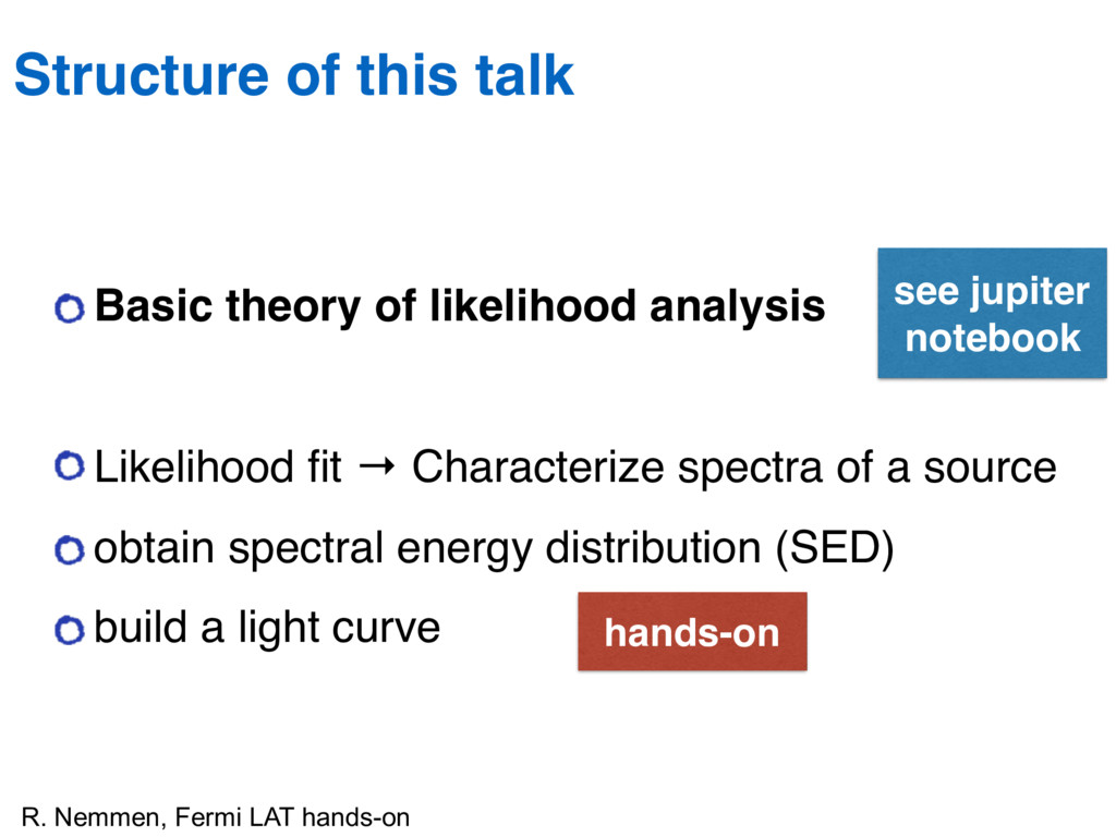
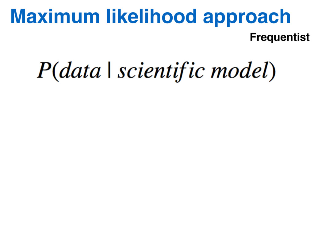
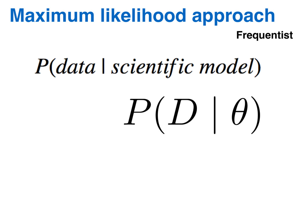
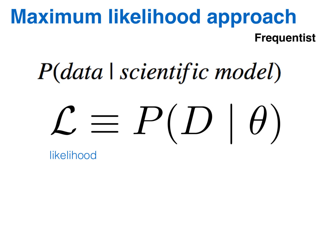
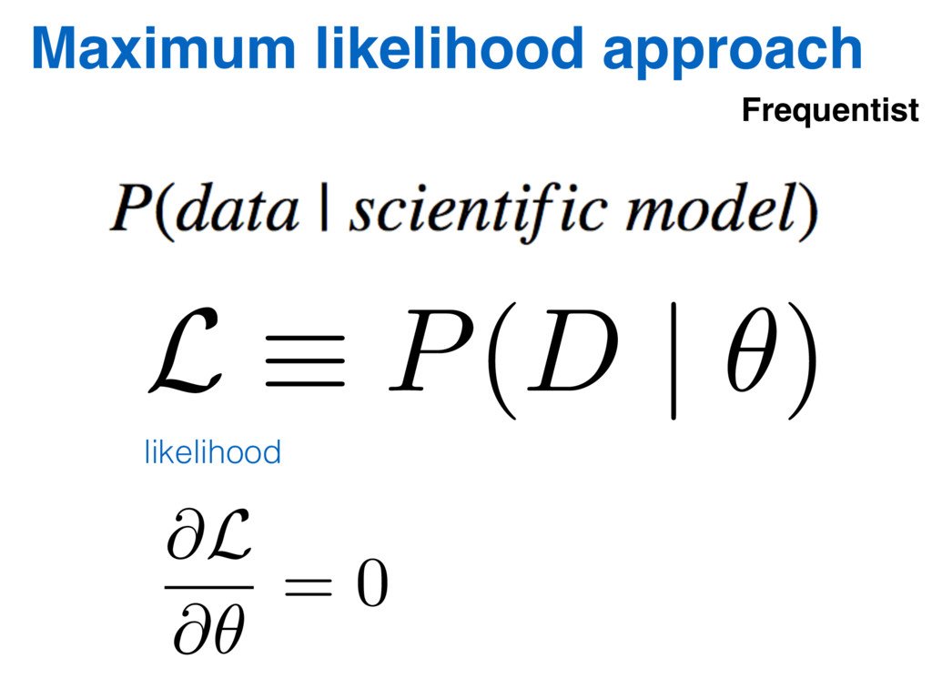
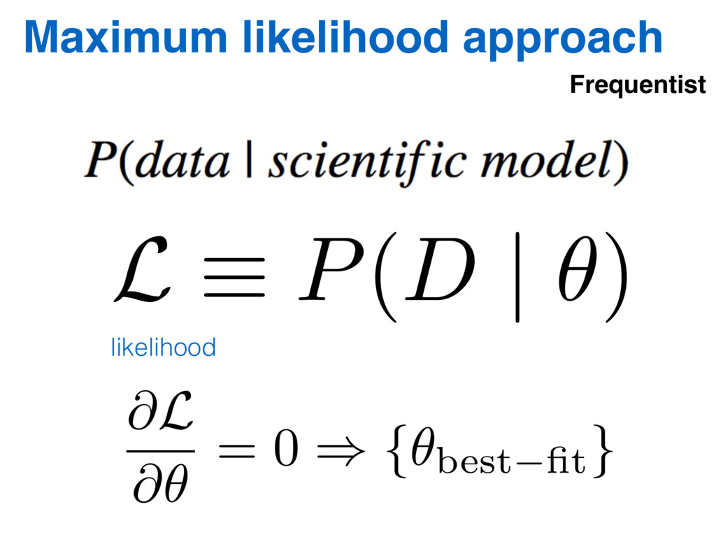
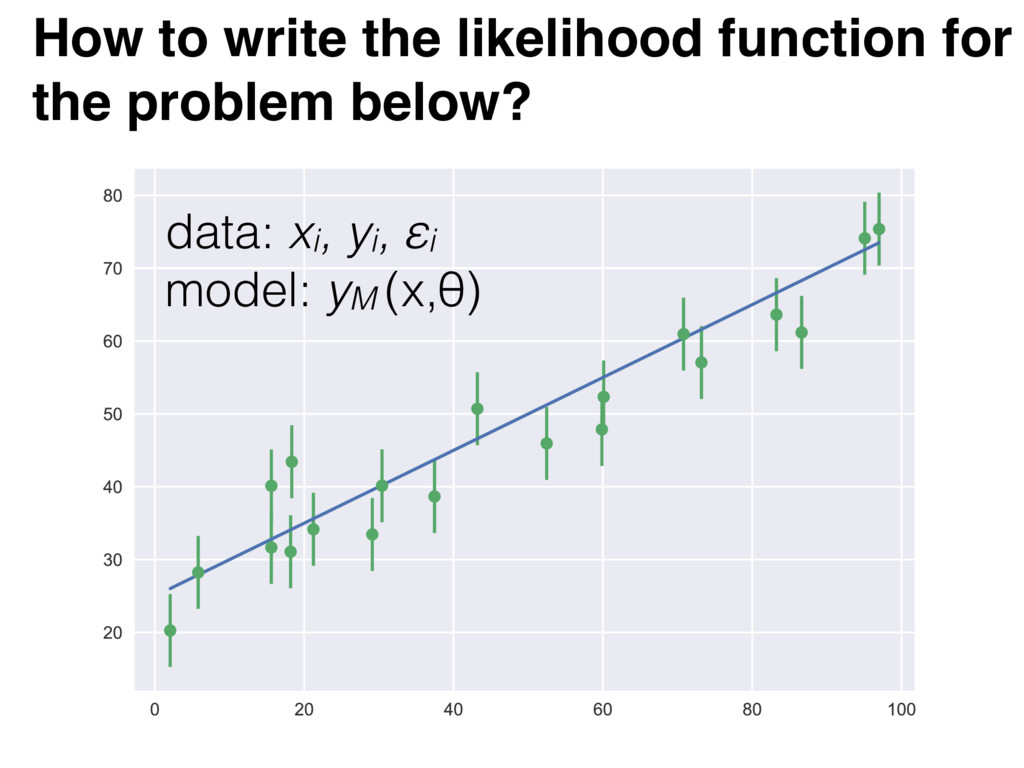
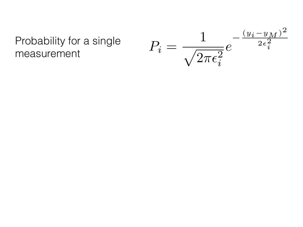
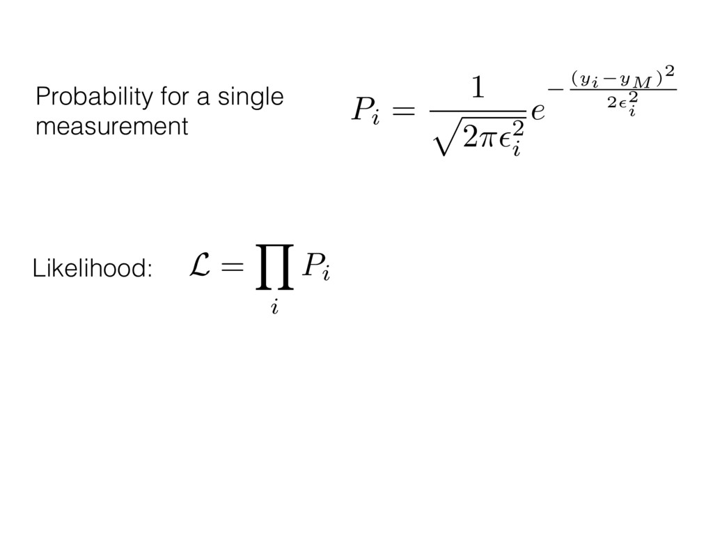
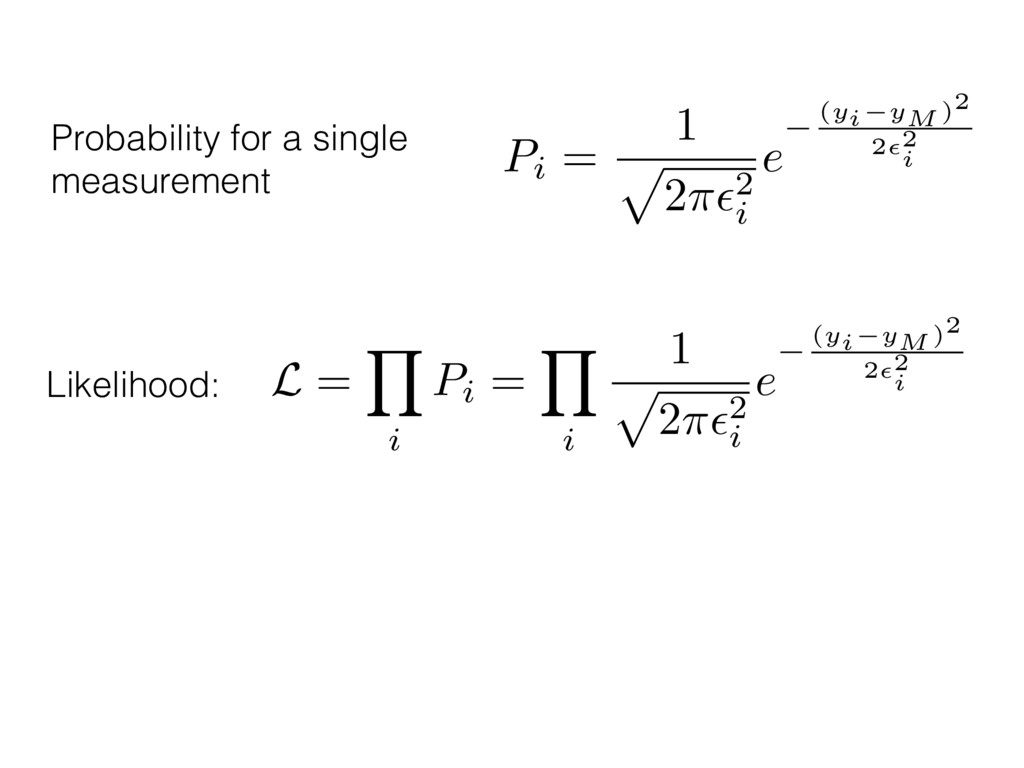
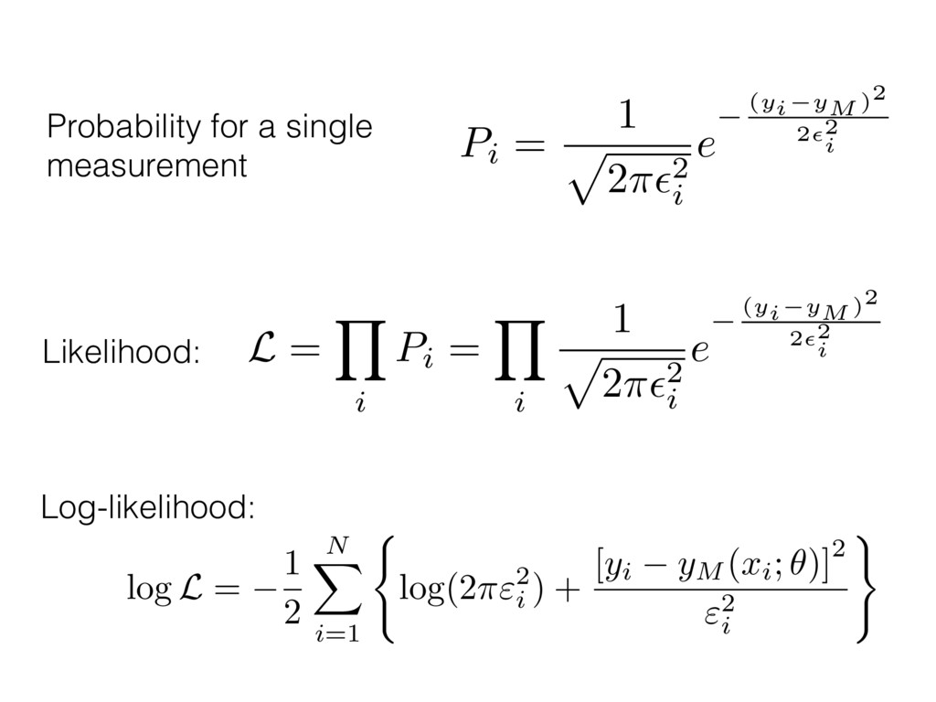
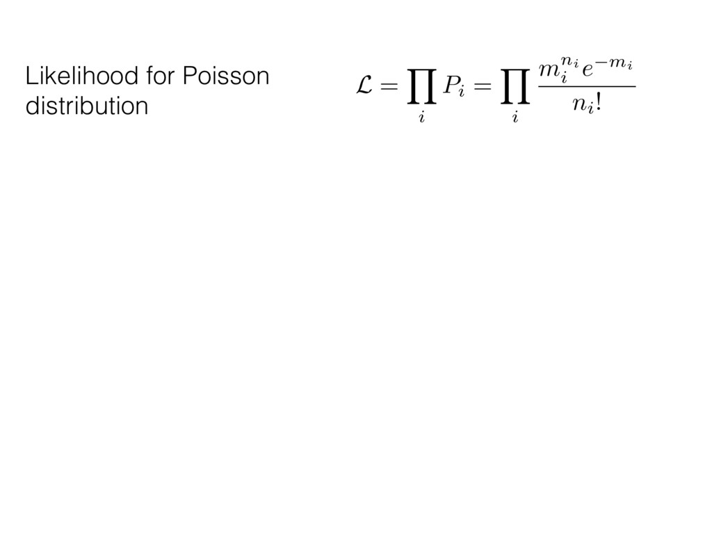
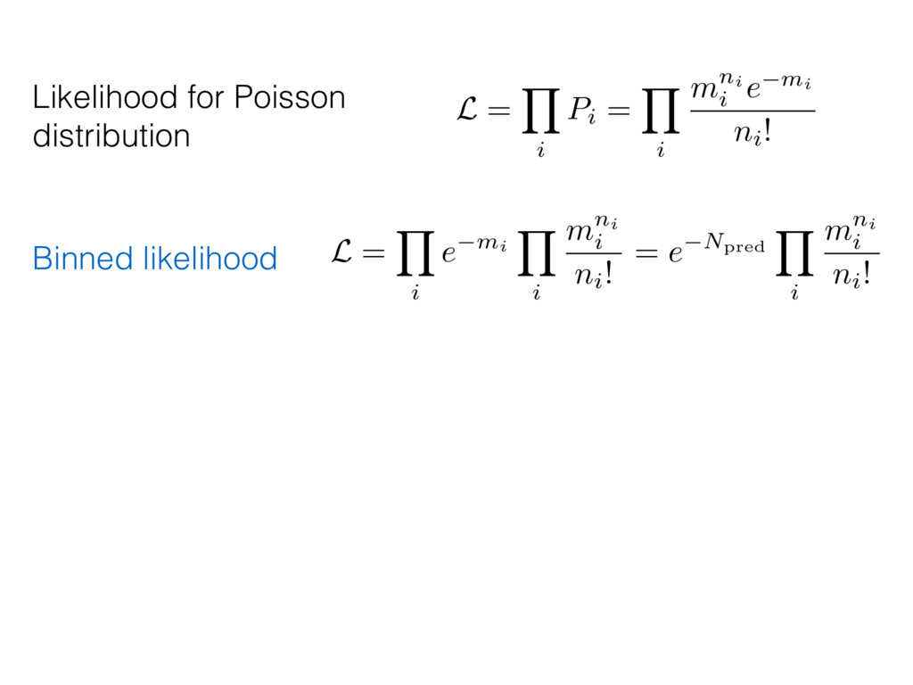
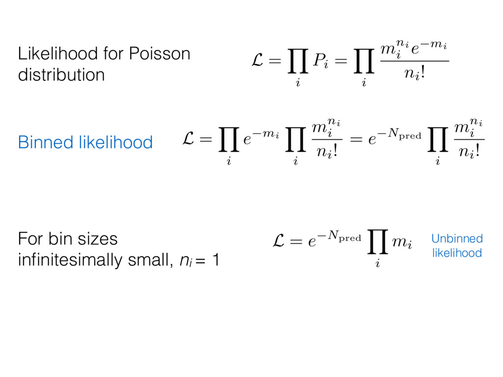
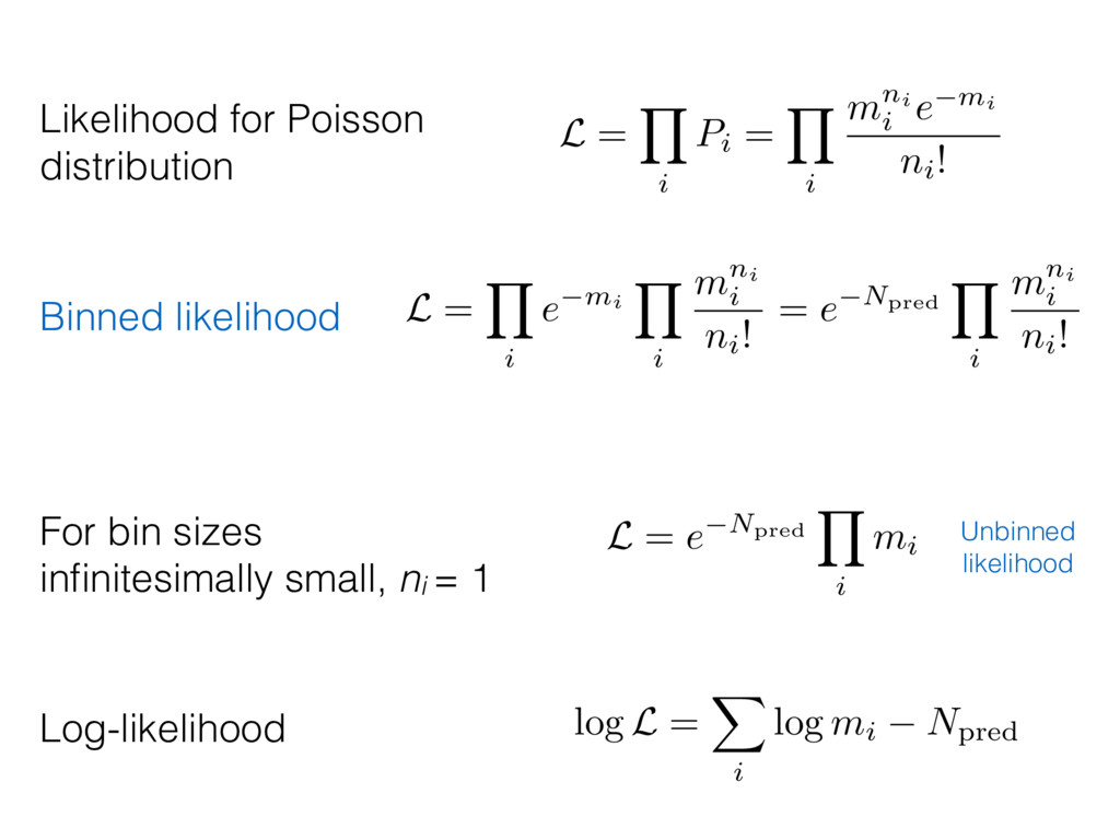
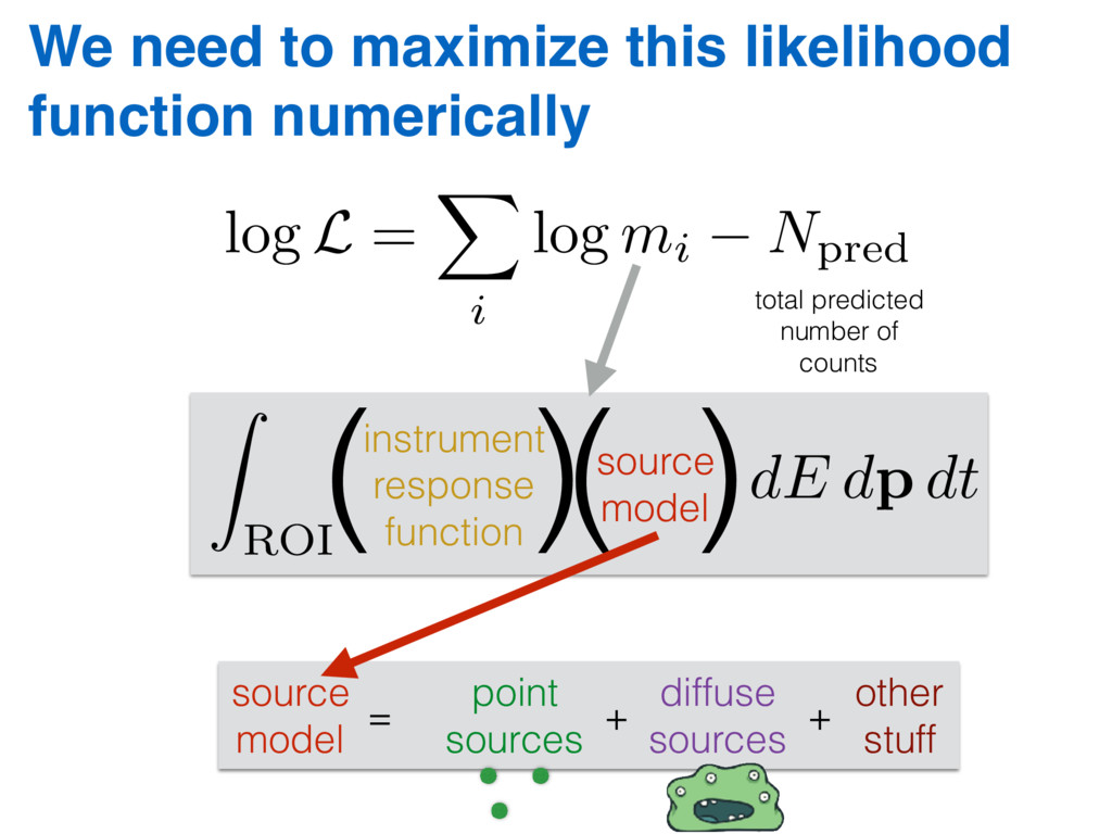
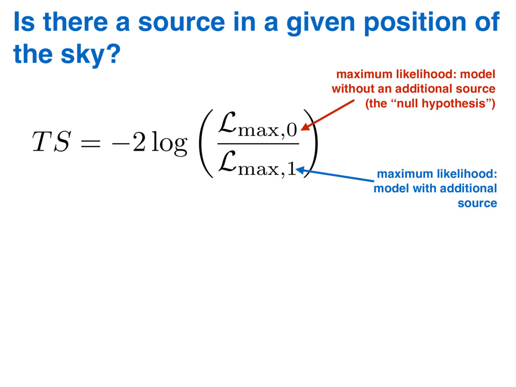
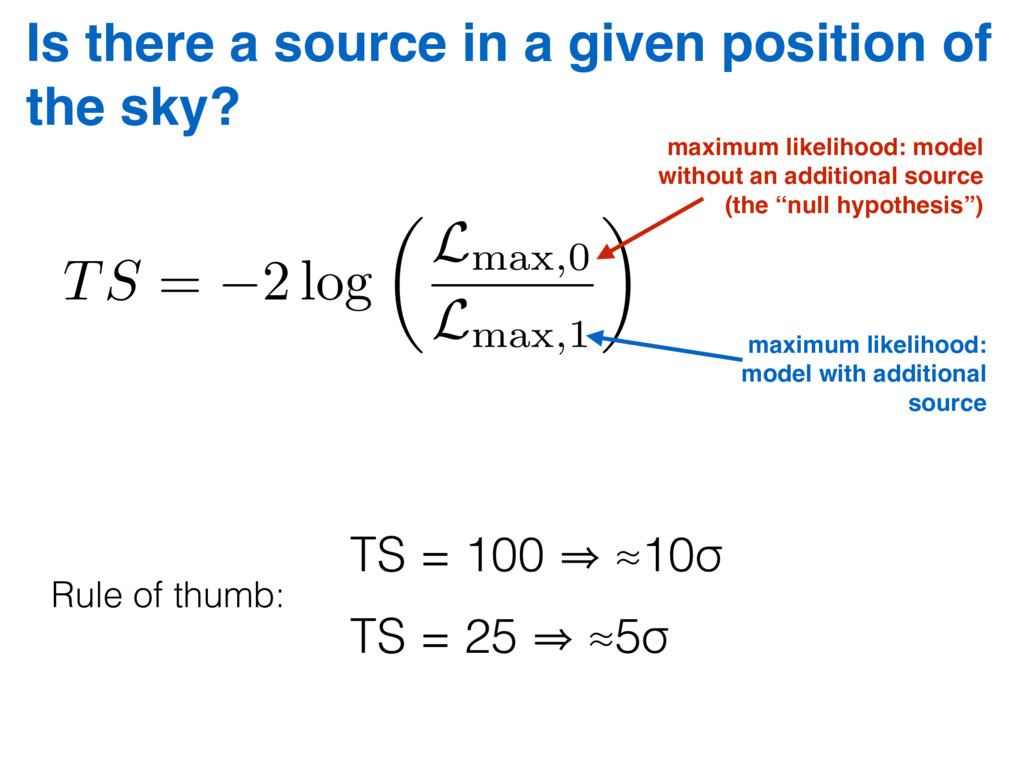
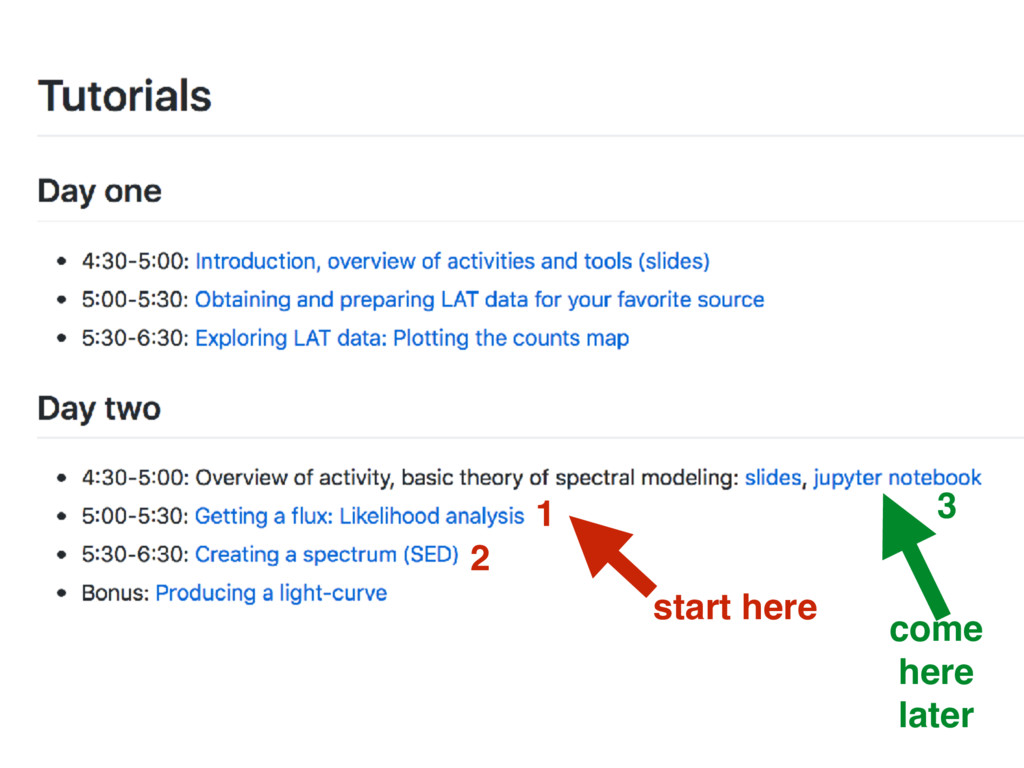
• Basic theory of likelihood analysis
• Likelihood fit → Characterize spectra of a source
• obtain spectral energy distribution (SED)
• build a light curve

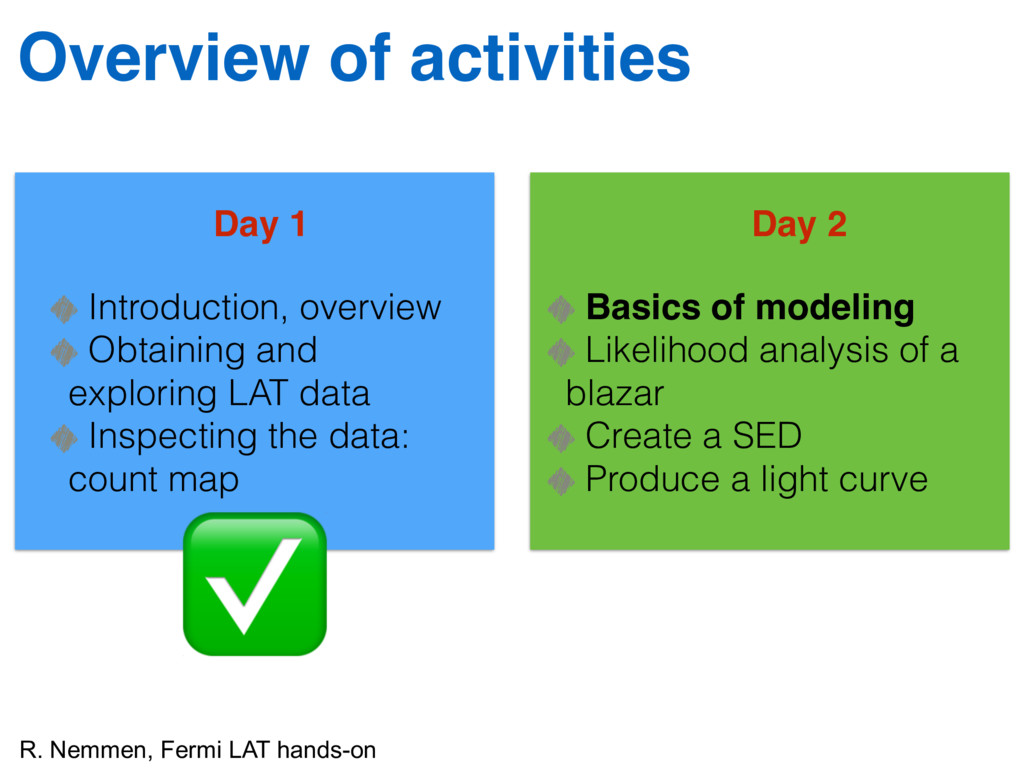
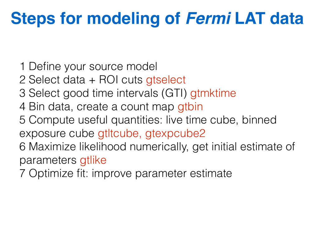
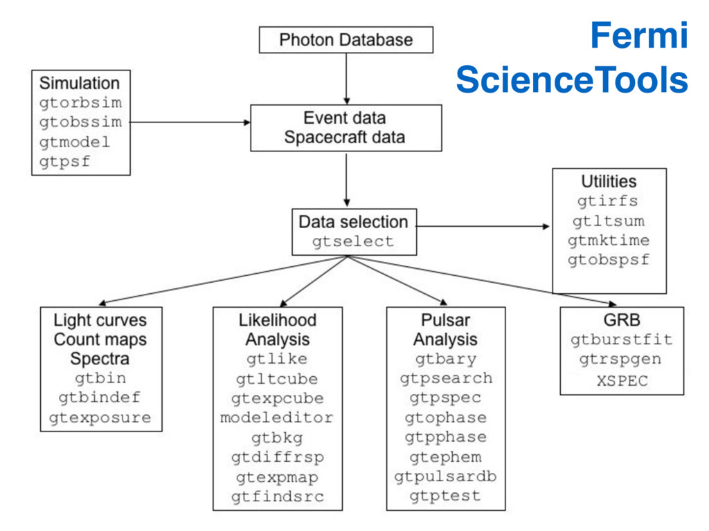
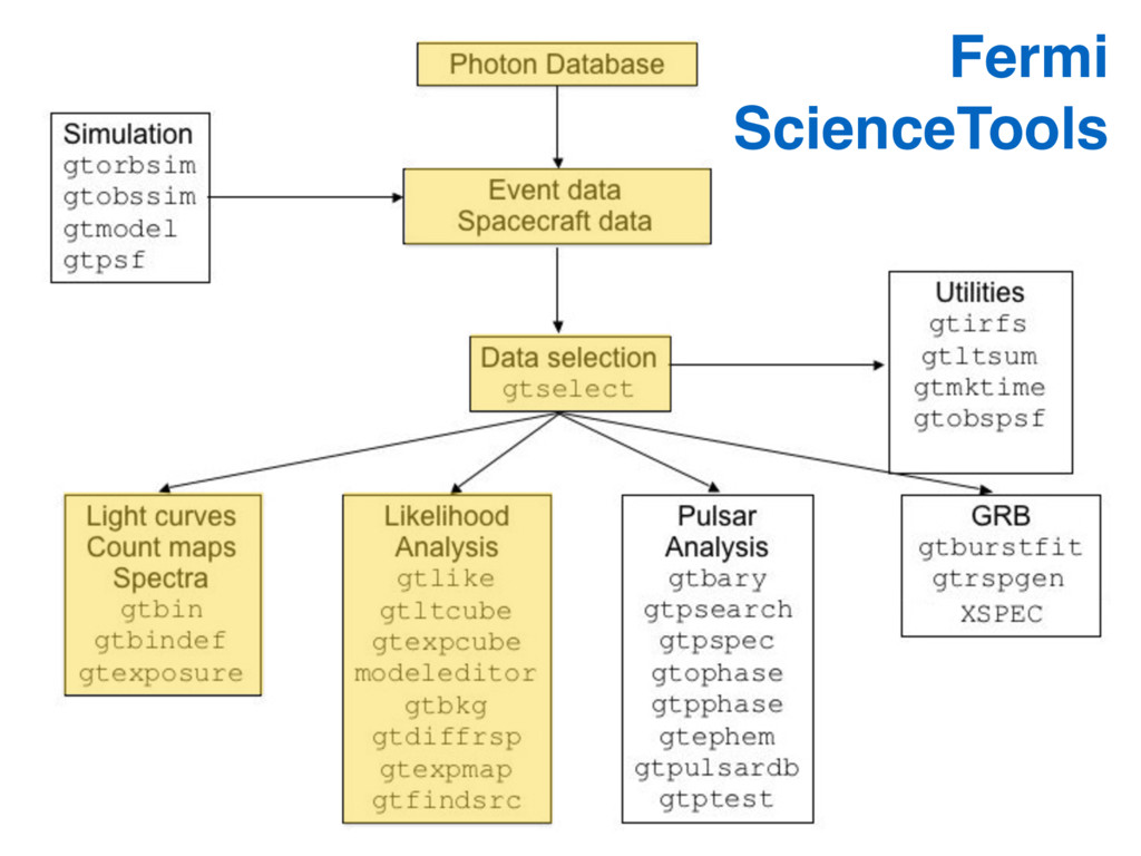
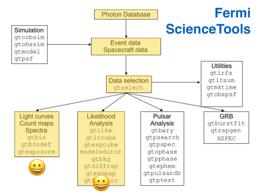
These are the tutorials for the hands on, practical session on the analysis of *Fermi* Large Area Telescope (aka LAT) gamma-ray observations for the São Paulo School of Advanced Science on High Energy and Plasma Astrophysics in the CTA Era. The goal of this activity is to get you started on the analysis of Fermi LAT data while giving you a concrete overview of the steps involved.

Link for material: https://github.com/rsnemmen/Fermi-LAT-tutorial

Transcript

1. Analysis of Fermi LAT data Analysis of Fermi LAT data Rodrigo Nemmen IAG USP May 24, 25 2017 High energy school @ IAG USP Likelihood tutorial
2. Overview of activities Day 1 Day 2 Introduction, overview Obtaining and exploring LAT data Inspecting the data: count map Basics of modeling Likelihood analysis of a blazar Create a SED Produce a light curve R. Nemmen, Fermi LAT hands-on ✅
3. Structure of this talk Basic theory of likelihood analysis Likelihood fit → Characterize spectra of a source obtain spectral energy distribution (SED) build a light curve see jupiter notebook hands-on R. Nemmen, Fermi LAT hands-on
4. Model fitting: given this model, what parameters best fit my data? Model selection: given two potential models, which better describes my data? Fundamental questions of science statistics R. Nemmen, Fermi LAT hands-on
5. Model fitting given this model, what parameters best fit my data?
6. Maximum likelihood approach Frequentist
7. Maximum likelihood approach Frequentist
8. L ⌘ P(D | ✓) Maximum likelihood approach Frequentist
9. L ⌘ P(D | ✓) likelihood Maximum likelihood approach Frequentist
10. L ⌘ P(D | ✓) likelihood Maximum likelihood approach Frequentist @L @✓ = 0 ) {✓best fit }
11. L ⌘ P(D | ✓) likelihood Maximum likelihood approach Frequentist @L @✓ = 0 ) {✓best fit }
12. How to write the likelihood function for the problem below? data: xi, yi, εi model: yM (x,θ)
13. Probability for a single measurement
14. Pi = 1 p 2⇡✏2 i e (yi yM )2 2✏2 i Probability for a single measurement
15. Pi = 1 p 2⇡✏2 i e (yi yM )2 2✏2 i Probability for a single measurement L = Y i Pi = Y i 1 p 2⇡✏2 i e (yi yM )2 2✏2 i Likelihood:
16. Pi = 1 p 2⇡✏2 i e (yi yM )2 2✏2 i Probability for a single measurement L = Y i Pi = Y i 1 p 2⇡✏2 i e (yi yM )2 2✏2 i Likelihood:
17. Pi = 1 p 2⇡✏2 i e (yi yM )2 2✏2 i Probability for a single measurement L = Y i Pi = Y i 1 p 2⇡✏2 i e (yi yM )2 2✏2 i Likelihood: Log-likelihood: log L = 1 2 N X i=1 ( log(2⇡" 2 i ) + [yi yM (xi; ✓)] 2 " 2 i )
18. What about Fermi LAT data?
19. Experiment counting events during a fixed interval: Poisson distribution
20. Experiment counting events during a fixed interval: Poisson distribution n: number of detected events m: expected number (model)
21. Experiment counting events during a fixed interval: Poisson distribution n: number of detected events m: expected number (model) P = mne m n! Probability of observing n events
22. Experiment counting events during a fixed interval: Poisson distribution Standard deviation = p n n: number of detected events m: expected number (model) P = mne m n! Probability of observing n events
23. Experiment counting events during a fixed interval: Poisson distribution P = mne m n! Standard deviation = p n
24. Experiment counting events during a fixed interval: Poisson distribution P = mne m n! Standard deviation = p n
25. Experiment counting events during a fixed interval: Poisson distribution P = mne m n! γ e- e+ γ e- e+ γ e- e+ Standard deviation = p n
26. Experiment counting events during a fixed interval: Poisson distribution P = mne m n! γ e- e+ γ e- e+ γ e- e+ Detected: n = 3 Standard deviation = p n
27. Experiment counting events during a fixed interval: Poisson distribution P = mne m n! γ e- e+ γ e- e+ γ e- e+ Detected: n = 3 Noise = sqrt(n) = 1.7 Standard deviation = p n
28. Experiment counting events during a fixed interval: Poisson distribution P = mne m n! γ e- e+ γ e- e+ γ e- e+ Detected: n = 3 Noise = sqrt(n) = 1.7 Expected: m = 2 Standard deviation = p n
29. L = Y i Pi = Y i mni i e mi ni! Likelihood for Poisson distribution
30. L = Y i Pi = Y i mni i e mi ni! Likelihood for Poisson distribution
31. L = Y i Pi = Y i mni i e mi ni! Likelihood for Poisson distribution L = Y i e mi Y i mni i ni! = e Npred Y i mni i ni! Binned likelihood
32. L = Y i Pi = Y i mni i e mi ni! Likelihood for Poisson distribution L = Y i e mi Y i mni i ni! = e Npred Y i mni i ni! Binned likelihood L = e Npred Y i mi For bin sizes infinitesimally small, ni = 1 Unbinned likelihood
33. L = Y i Pi = Y i mni i e mi ni! Likelihood for Poisson distribution L = Y i e mi Y i mni i ni! = e Npred Y i mni i ni! Binned likelihood log L = X i log mi Npred Log-likelihood L = e Npred Y i mi For bin sizes infinitesimally small, ni = 1 Unbinned likelihood
34. log L = X i log mi Npred We need to maximize this likelihood function numerically total predicted number of counts Z ROI dE dp dt Z ROI dE dp dt instrument response function source model ( )( ) source model = point sources diffuse sources other stuff + +
35. Model selection given two potential models, which better describes my data?
36. Is there a source in a given position of the sky? TS = 2 log ✓ L max , 0 L max , 1 ◆ maximum likelihood: model with additional source maximum likelihood: model without an additional source (the “null hypothesis”)
37. Is there a source in a given position of the sky? TS = 2 log ✓ L max , 0 L max , 1 ◆ maximum likelihood: model with additional source maximum likelihood: model without an additional source (the “null hypothesis”) TS = 100 㱺 ≈10σ TS = 25 㱺 ≈5σ Rule of thumb:
38. Hands-on activity
39. 1 Define your source model 2 Select data + ROI cuts gtselect 3 Select good time intervals (GTI) gtmktime 4 Bin data, create a count map gtbin 5 Compute useful quantities: live time cube, binned exposure cube gtltcube, gtexpcube2 6 Maximize likelihood numerically, get initial estimate of parameters gtlike 7 Optimize fit: improve parameter estimate Steps for modeling of Fermi LAT data
40. Fermi ScienceTools
41. Fermi ScienceTools
42. Fermi ScienceTools
43. Python wrappers make analysis of Fermi data much easier: Enrico and fermipy We will use Enrico: http://enrico.readthedocs.io/en/latest/
44. Tutorial website https://github.com/rsnemmen/Fermi-LAT-tutorial
45. start here come here later 1 2 3
46. Please do not download large files during the tutorial or the WIFI network will overload We will distribute the software and data you need via USB sticks
47. Github Twitter Web E-mail Bitbucket Facebook Blog figshare rodrigo.nemmen@iag.usp.br http://rodrigonemmen.com @nemmen rsnemmen http://facebook.com/rodrigonemmen nemmen http://astropython.blogspot.com http://bit.ly/2fax2cT