SIAM

Advances in the numerical solution of the time-domain electromagnetic inverse problem

(Talk presented at the SIAM Geosciences 2017, Erlangen)

Transcript

1. Advances in the numerical solution of the time–domain electromagnetic inverse problem R.–U. Börner1, F. Eckhofer2, and M. Helm2 1 Institute of Geophysics and Geoinformatics 2 Institute of Numerical Analysis and Optimization TU Bergakademie Freiberg (Germany) SIAM Conference on Mathematical and Computational Issues in the Geosciences Erlangen (Germany) · September 11-14, 2017
2. Table of contents 1. Introduction 2. The inverse problem 3. Review of numerical approaches 4. Examples 5. Summary 1
3. Introduction
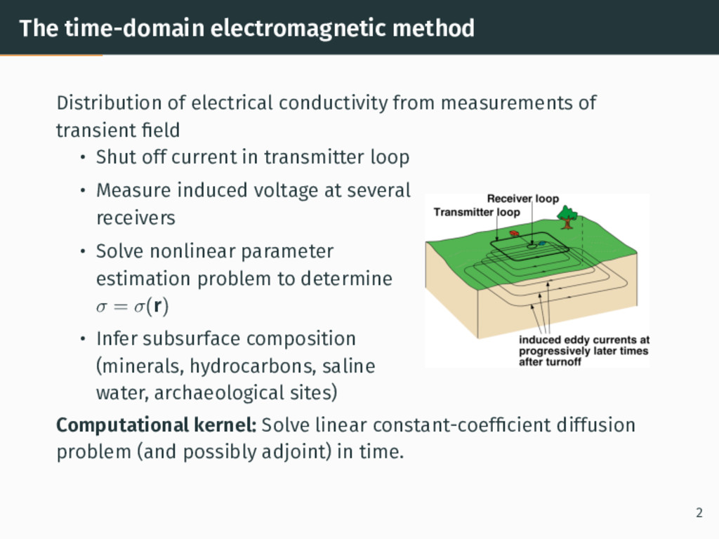
4. The time-domain electromagnetic method Distribution of electrical conductivity from measurements of transient field • Shut off current in transmitter loop • Measure induced voltage at several receivers • Solve nonlinear parameter estimation problem to determine σ = σ(r) • Infer subsurface composition (minerals, hydrocarbons, saline water, archaeological sites) Computational kernel: Solve linear constant-coefficient diffusion problem (and possibly adjoint) in time. 2
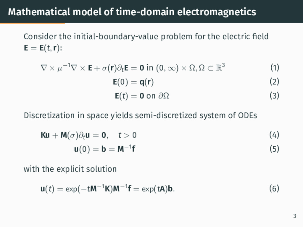
5. Mathematical model of time-domain electromagnetics Consider the initial-boundary-value problem for the electric field E = E(t, r): ∇ × µ−1 ∇ × E + σ(r)∂t E = 0 in (0, ∞) × Ω, Ω ⊂ R3 (1) E(0) = q(r) (2) E(t) = 0 on ∂Ω (3) Discretization in space yields semi-discretized system of ODEs Ku + M(σ)∂t u = 0, t > 0 (4) u(0) = b = M−1f (5) with the explicit solution u(t) = exp(−tM−1K)M−1f = exp(tA)b. (6) 3
6. Example: Distribution of ∂t Bz(t) = −[∇ × E(t)]z Homogeneous halfspace, early time, t ≈ 8e-6 s max. induced voltage ≈ -4.7e-8 V/m2 4
7. Example: Distribution of ∂t Bz(t) = −[∇ × E(t)]z Homogeneous halfspace, intermediate time, t ≈ 6e-5 s max. induced voltage ≈ -6.4e-10 V/m2 4
8. Example: Distribution of ∂t Bz(t) = −[∇ × E(t)]z Homogeneous halfspace, late time, t ≈ 1e-3 s max. induced voltage ≈ -6.8e-12 V/m2 4
9. The inverse problem
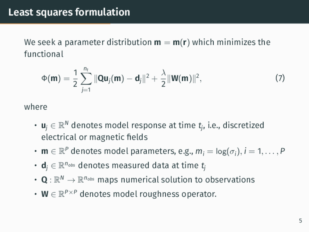
10. Least squares formulation We seek a parameter distribution m = m(r) which minimizes the functional Φ(m) = 1 2 nt ∑ j=1 ∥Quj(m) − dj∥2 + λ 2 ∥W(m)∥2 , (7) where • uj ∈ RN denotes model response at time tj , i.e., discretized electrical or magnetic fields • m ∈ RP denotes model parameters, e.g., mi = log(σi), i = 1, . . . , P • dj ∈ Rnobs denotes measured data at time tj • Q : RN → Rnobs maps numerical solution to observations • W ∈ RP×P denotes model roughness operator. 5
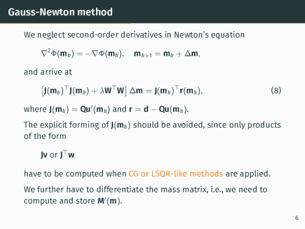
11. Gauss-Newton method We neglect second-order derivatives in Newton’s equation ∇2 Φ(mk) = −∇Φ(mk), mk+1 = mk + ∆m, and arrive at [ J(mk)⊤J(mk) + λW⊤W ] ∆m = J(mk)⊤r(mk), (8) where J(mk) = Qu′(mk) and r = d − Qu(mk). The explicit forming of J(mk) should be avoided, since only products of the form Jv or J⊤w have to be computed when CG or LSQR-like methods are applied. We further have to differentiate the mass matrix, i.e., we need to compute and store M′(m). 6
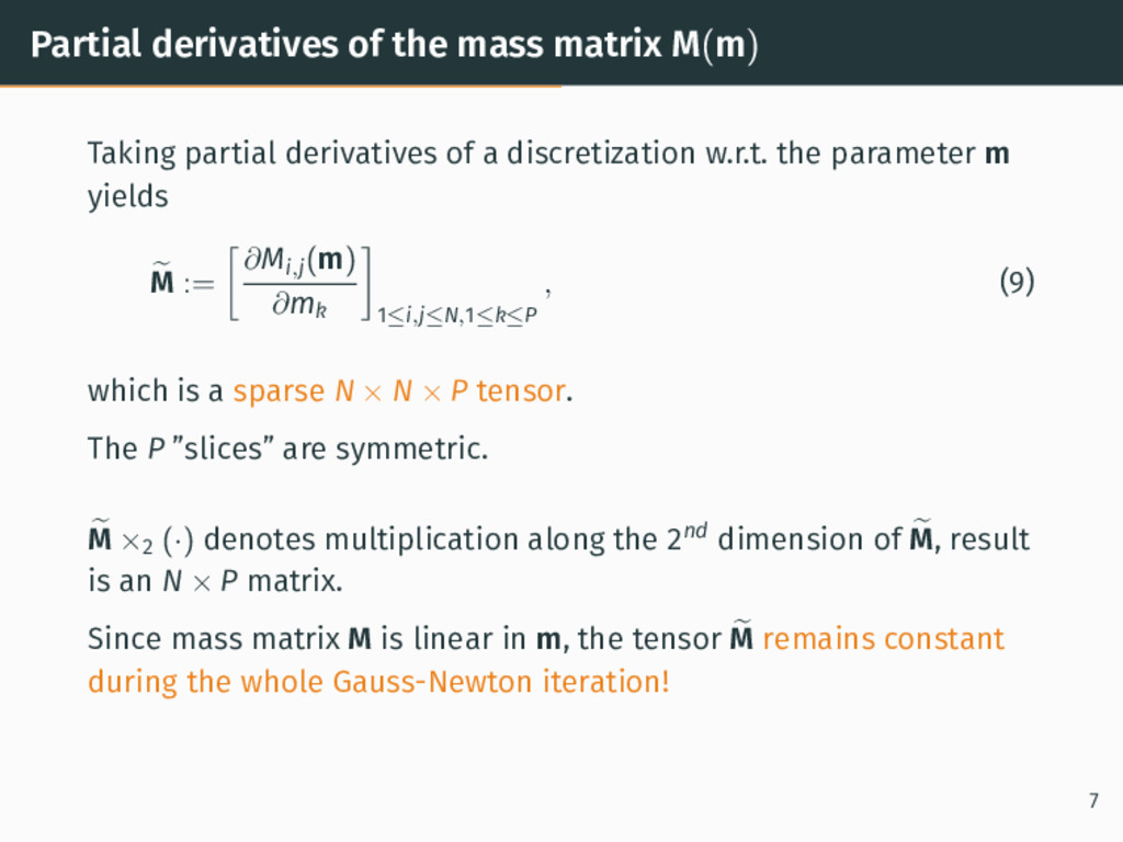
12. Partial derivatives of the mass matrix M(m) Taking partial derivatives of a discretization w.r.t. the parameter m yields M := [ ∂Mi,j(m) ∂mk ] 1≤i,j≤N,1≤k≤P , (9) which is a sparse N × N × P tensor. The P ”slices” are symmetric. M ×2 (·) denotes multiplication along the 2nd dimension of M, result is an N × P matrix. Since mass matrix M is linear in m, the tensor M remains constant during the whole Gauss-Newton iteration! 7
13. Review of numerical approaches
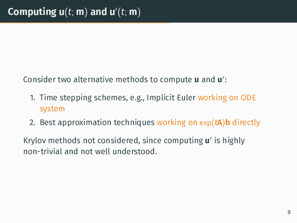
14. Computing u(t; m) and u′(t; m) Consider two alternative methods to compute u and u′: 1. Time stepping schemes, e.g., Implicit Euler working on ODE system 2. Best approximation techniques working on exp(tA)b directly Krylov methods not considered, since computing u′ is highly non-trivial and not well understood. 8
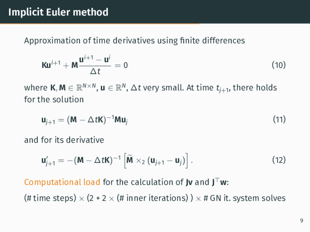
15. Implicit Euler method Approximation of time derivatives using finite differences Kui+1 + M ui+1 − ui ∆t = 0 (10) where K, M ∈ RN×N, u ∈ RN, ∆t very small. At time tj+1 , there holds for the solution uj+1 = (M − ∆tK)−1Muj (11) and for its derivative u′ j+1 = −(M − ∆tK)−1 [ M ×2 (uj+1 − uj) ] . (12) Computational load for the calculation of Jv and J⊤w: (# time steps) × (2 + 2 × (# inner iterations) ) × # GN it. system solves 9
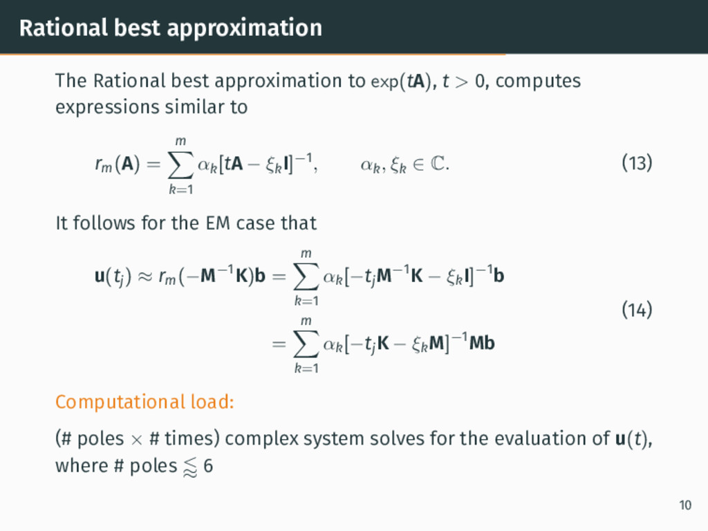
16. Rational best approximation The Rational best approximation to exp(tA), t > 0, computes expressions similar to rm(A) = m ∑ k=1 αk[tA − ξk I]−1 , αk, ξk ∈ C. (13) It follows for the EM case that u(tj) ≈ rm(−M−1K)b = m ∑ k=1 αk[−tj M−1K − ξk I]−1b = m ∑ k=1 αk[−tj K − ξk M]−1Mb (14) Computational load: (# poles × # times) complex system solves for the evaluation of u(t), where # poles ⪅ 6 10
17. Rational best approximation To compute Jv and J⊤w, we obtain Jv = Qu′(m)v = m ∑ k=1 αkξk Q[−tj K − ξk M]−1 { M ×2 [−tj K − ξk M]−1f } N×P v (15) J⊤w = (w⊤J)⊤ = m ∑ k=1 αkξk { M ×2 [−tj K − ξk M]−1f }⊤ P×N [−tj K − ξk M]−1Q⊤w (16) Computational load: (2 + # inner it.) × (# poles) × (# times) × (# GN it.) complex system solves + 2 (# inner it.) × (# poles) × (# times) × (# GN it.) matrix-vector multiplications for the computation of parameter updates 11
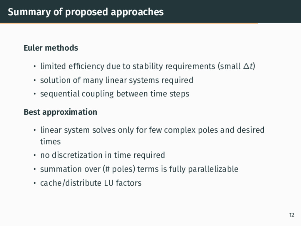
18. Summary of proposed approaches Euler methods • limited efficiency due to stability requirements (small ∆t) • solution of many linear systems required • sequential coupling between time steps Best approximation • linear system solves only for few complex poles and desired times • no discretization in time required • summation over (# poles) terms is fully parallelizable • cache/distribute LU factors 12
19. Examples
20. Minimal toy example: Best approximation variant TEM data: 1 transmitter source, 10 receivers (# obs), 31 times (# times) true model 0 100 200 300 400 500 600 r in m 0 50 100 150 200 250 300 z in m 3.0 2.5 2.0 1.5 1.0 0.5 0.0 log( /(S/m)) 13
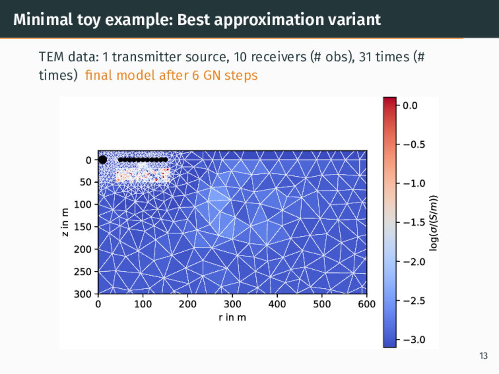
21. Minimal toy example: Best approximation variant TEM data: 1 transmitter source, 10 receivers (# obs), 31 times (# times) final model after 6 GN steps 0 100 200 300 400 500 600 r in m 0 50 100 150 200 250 300 z in m 3.0 2.5 2.0 1.5 1.0 0.5 0.0 log( /(S/m)) 13
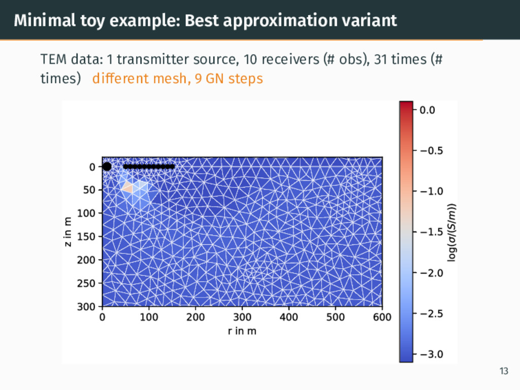
22. Minimal toy example: Best approximation variant TEM data: 1 transmitter source, 10 receivers (# obs), 31 times (# times) different mesh, 9 GN steps 0 100 200 300 400 500 600 r in m 0 50 100 150 200 250 300 z in m 3.0 2.5 2.0 1.5 1.0 0.5 0.0 log( /(S/m)) 13
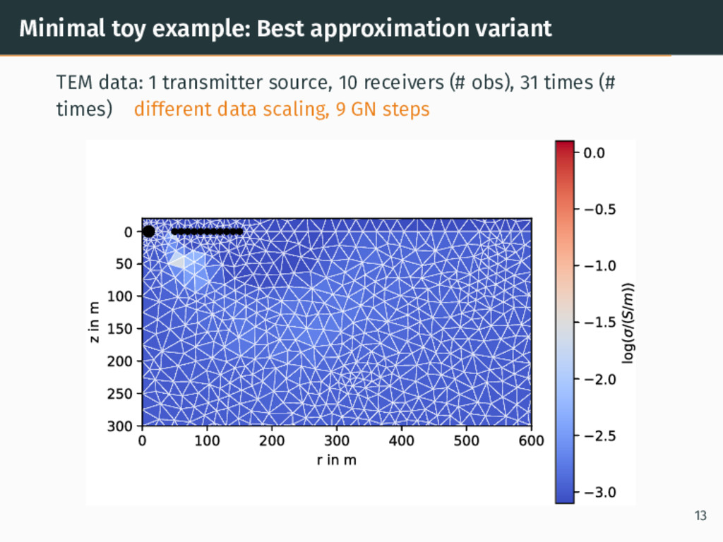
23. Minimal toy example: Best approximation variant TEM data: 1 transmitter source, 10 receivers (# obs), 31 times (# times) different data scaling, 9 GN steps 0 100 200 300 400 500 600 r in m 0 50 100 150 200 250 300 z in m 3.0 2.5 2.0 1.5 1.0 0.5 0.0 log( /(S/m)) 13
24. Summary
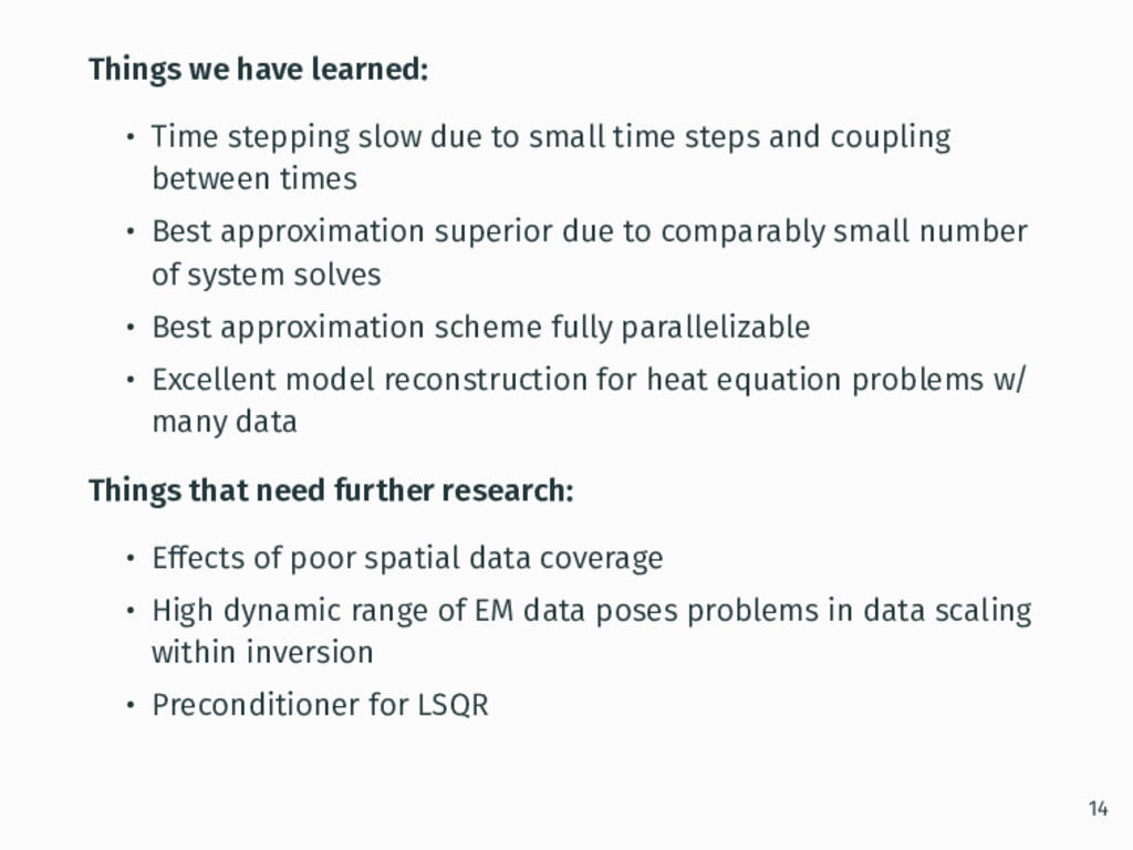
25. Things we have learned: • Time stepping slow due to small time steps and coupling between times • Best approximation superior due to comparably small number of system solves • Best approximation scheme fully parallelizable • Excellent model reconstruction for heat equation problems w/ many data Things that need further research: • Effects of poor spatial data coverage • High dynamic range of EM data poses problems in data scaling within inversion • Preconditioner for LSQR 14
26. Thank you for your attention! 14