Tour de Force: Stream Based Textanalysis

Stream Based Textanalysis with Elasticsearch, Spark and R

Transcript

1. Tour de Force: Stream Based Textanalysis Hendrik Saly Stefan Siprell
2. 2 Motivation zum Vortrag Machine Learning ist auch nur Source Code Abbauen von Berührungsängsten Die Tools hierfür sind schon alle da
3. 3 This is not •  First implementations written in R •  Attempt was OK, but not really good •  Let us talk about R, Spark, LingPipe & ELK!
4. 4 Agenda: Wild Ride CRISP For Data Modelling •  Demo: Text Classification on Twitter using Spark, LingPipe & Kibana •  Intercept: Breakfast Club with R We are running out of time!
5. 5 Cross Industry Standard Process for Data Mining What do we want to achieve? Explorative Analysis of the data, Ensure Data Quality Structure and Clean Data Choose and configure Algorithms Validate the model Integrate with other systems
6. 6 Business Understanding
7. 7 How can a machine make sense of this? What club is the user talking about? Is his statement positiv or negativ? What do we know about the author?
8. 8 We want to analyze the text to find out, which club the tweet is about. We can use following bits of information •  Clubtitle with inoffical aliases •  Player Names •  Dialect •  Relevant Events In addition we want to figure out the emotional bias To achieve this we use the following algortihms •  Document Classification •  Sentiment Detection Two Mechanisms to understand the content
9. 9 Data Understanding & Data Preparation
10. 10 We recommend the following tools for that: " R – You need some experience but then its a pretty lightweight yet powerful tool " ELK – Easy to setup and easy to use - also for unexperineced users. Great for getting an explorative understanding of your data Tools
11. 11 First Tool - R R is language and runtime for statistcs and charting It‘s great for getting a quick overview of your data
12. 12 gradyear,gender,age,friends,basketball,football,soccer,softball,volleyball,swimming, cheerleading,baseball,tennis,sports,cute,sex,sexy,hot,kissed,dance,band,marching ,music,rock,god,church,jesus,bible,hair,dress,blonde,mall,shopping,clothes,holli ster,abercrombie,die,death,drunk,drugs 2006,M, 18.982,7,0,0,0,0,0,0,0,0,0,0,0,0,0,0,0,1,0,0,0,0,0,0,0,0,0,0,0,0,0,0,0,0,0,0,0,0 2006,F, 18.801,0,0,1,0,0,0,0,0,0,0,0,1,0,0,0,0,0,0,0,2,2,1,0,0,0,6,4,0,1,0,0,0,0,0,0,0,0 2006,M, 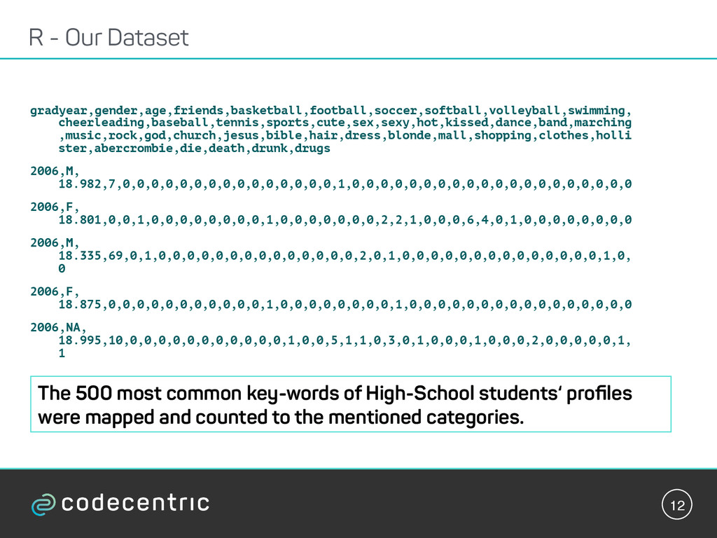18.335,69,0,1,0,0,0,0,0,0,0,0,0,0,0,0,0,0,2,0,1,0,0,0,0,0,0,0,0,0,0,0,0,0,0,1,0, 0 2006,F, 18.875,0,0,0,0,0,0,0,0,0,0,0,1,0,0,0,0,0,0,0,0,1,0,0,0,0,0,0,0,0,0,0,0,0,0,0,0,0 2006,NA, 18.995,10,0,0,0,0,0,0,0,0,0,0,0,1,0,0,5,1,1,0,3,0,1,0,0,0,1,0,0,0,2,0,0,0,0,0,1, 1 R - Our Dataset The 500 most common key-words of High-School students‘ profiles were mapped and counted to the mentioned categories.
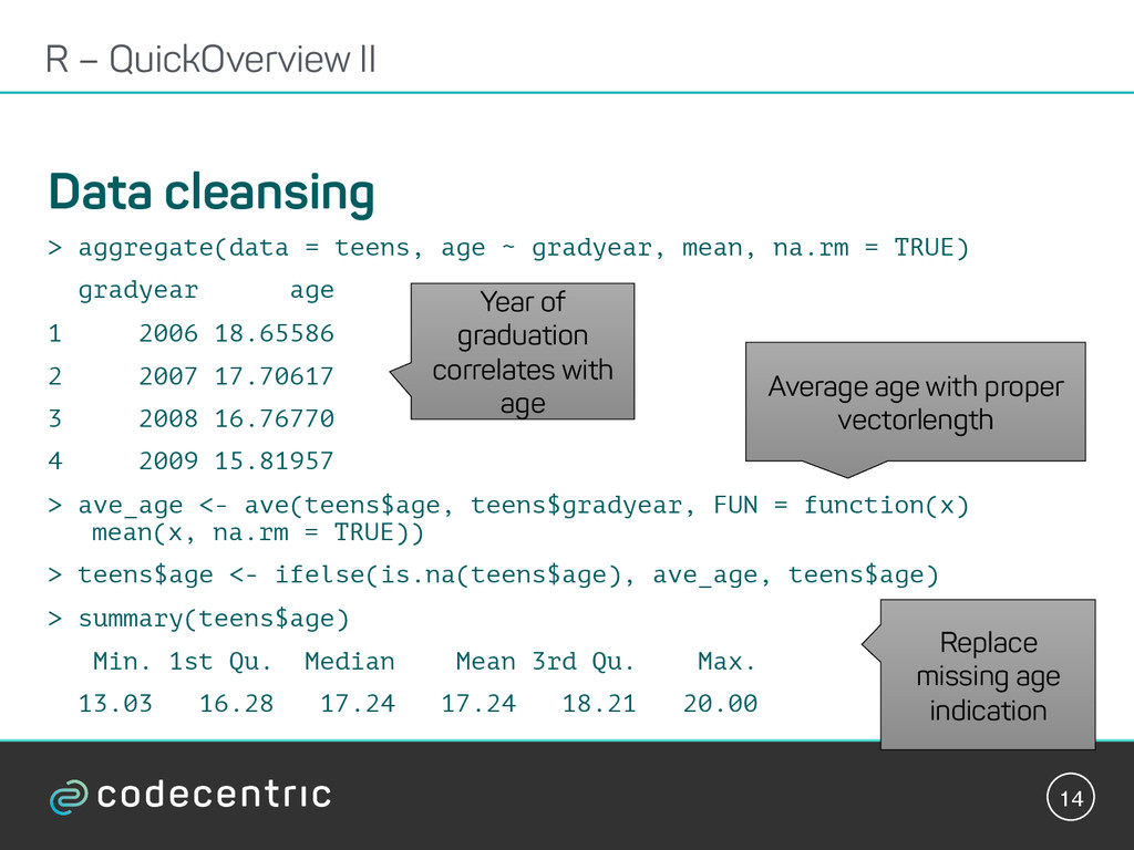
13. 13 Load data teens <- read.csv("~/Downloads/snsdata.csv") Print it > table (teens$gender) F M 22054 5222 > summary(teens$age) Min. 1st Qu. Median Mean 3rd Qu. Max. NA's 3.086 16.310 17.290 17.990 18.260 106.900 5086 R – QuickOverview Maybe too young?!? Maybe too old?!? Where are the boys?
14. 14 Data cleansing > aggregate(data = teens, age ~ gradyear, mean, na.rm = TRUE) gradyear age 1 2006 18.65586 2 2007 17.70617 3 2008 16.76770 4 2009 15.81957 > ave_age <- ave(teens$age, teens$gradyear, FUN = function(x) mean(x, na.rm = TRUE)) > teens$age <- ifelse(is.na(teens$age), ave_age, teens$age) > summary(teens$age) Min. 1st Qu. Median Mean 3rd Qu. Max. 13.03 16.28 17.24 17.24 18.21 20.00 R – QuickOverview II Year of graduation correlates with age Average age with proper vectorlength Replace missing age indication
15. 15 Data clustering > interests <- teens[5:40] > interests_z <- as.data.frame(lapply(interests, scale)) > teen_clusters <- kmeans(interests_z, 5) Why 5 clusters? R – QuickOverview III
16. 16 Data cleansing basketball football soccer softball volleyball swimming 1 0.3427687 0.36148309 0.12406954 0.16495749 0.11129383 0.27097377 2 0.5347402 0.49217281 0.29328529 0.37835496 0.38660379 0.29699406 3 -0.1197076 0.03407084 -0.07534803 -0.01857530 -0.08231183 0.04443602 4 0.1600123 0.23641736 0.10385512 0.07232021 0.18897158 0.23970234 5 -0.1659121 -0.16399209 -0.08820562 -0.11448214 -0.11651468 -0.10635639 hollister abercrombie die death drunk drugs 1 0.16213333 0.26454350 1.71491556 0.93757803 1.901120381 2.72769246 2 -0.05574868 -0.07262787 0.03919937 0.12049381 -0.009236523 -0.06055113 3 -0.16931294 -0.14756789 -0.02295448 0.02216690 -0.086897407 -0.08524621 4 4.15218436 3.96493810 0.04347597 0.09857501 0.035614771 0.03443294 5 -0.15510547 -0.14858519 -0.09435262 -0.08324495 -0.087243227 -0.11294654 R – QuickOverview II
17. 17 Which 5 Cluster? R – QuickOverview III Criminal Sports, Sex, Sexy, Hot, Kissed, Danced, Music, Band, Die, Death, Drugs, Drunk Athlete Basketball, Football, Soccer, Softball, Volleyball, Baseball, Sports, God, Church, Jesus, Bible Princess Swimming, Cheerleading, Cute, Sexy, Hot, Dance, Dress, Hair, Mall, Hollister, Abercrombie, Shopping, Clothes Brains Band, Marching, Music, Rock Basket Case
18. 18 Example comes from:
19. 19 Spark is the „swiss army knife“ for Data and can be used for: •  ETL – Transform many different data formats and store them in RDBMS and NoSQL databases. SQL – Access arbitratry datasources via SQL. •  R – Access Spark RDD‘s natively from R •  Streaming – Also handles data streams •  Machine Learning – Spark integrates well with Machine Learing Spark
20. 20 We have collected almost 1 Mio Tweets as flat files and we want them load into Elasticsearch Within Elasticsearch we want to analyse the data in an explorative manner, process and store them. With Spark we can do this with only 47 lines of code! Spark for loading data
21. 21 SparkConf*sparkConfig*=*new*SparkConf();* sparkConfig.setMaster("local[3]").setAppName("ES*Loader");* sparkConfig.set("es.nodes",*“XXX.euEwestE1.aws.found.io:9200");* * * Spark configuration
22. 22 try*(JavaSparkContext*sc*=*new*JavaSparkContext(sparkConfig))*{* ******ListObjectsRequest*request*=*new*ListObjectsRequest();* ******request.setBucketName(s3config.getBucketName());* ******request.setPrefix(s3config.getPrefix());* ******request.setMaxKeys(s3config.getMaxKeys());* ******ObjectListing*objs*=*s3.listObjects(request);* ******JavaRDD<String>*rdd*=* sc.parallelize(objs.getObjectSummaries().stream().map(entry*)>* entry.getKey()).collect(Collectors.toList()))* **********.flatMap(key*)>*FileContentLoader.loadContents(s3,* s3config.getBucketName(),*key));* *JavaEsSpark.saveJsonToEs(rdd,*"tweets/tweet");* }* Load 1000 Gzip Archives with 1000 Tweets each from S3 into Elasticsearch
23. 23 ELK Dashboards
24. 24 Modeling & Evaluation
25. 25 Machine Learning – Unsupervised Learning Unsupervised Learning •  Find patterns in arbitrary data (isolate them from noise) •  Patterns are not predefined •  Used for segmentation and compression of data •  Examples: k-means, Hierarchical, etc.
26. 26 Machine Learning – Supervised Learning Supervised Learning •  Training is based on features and well defined categories •  Criterias are defined upfront •  Data is classified automatically by applying learnt rules •  Examples: Decision Trees, Naive Bayes, Neuronal Networks
27. 27 Machine Learning – Reinforcement Learning Reinforcement Learning •  Online Training •  Succes or failures has to be recognizable •  The system does not know why something works. It only does that it works (or not). •  Underlying base is often the Markov Decision Process
28. 28 Our classifiers are based upon naive Bayes and/or Support Vector‘s, which need a training run. So we have to build a training data set first. That might be easy. For that we map the most common hashtags (Kibana) to soccer teams (Spark) and store the results back to Elasticsearch. Supervised Learning
29. 29 private*static*String[][]*clubs*=* ******new*String[][]*{{"FC*Bayern",*"Schweinsteiger",* "BastianSchweinsteiger",*"FCBayern",*"BayernMünchen",* "Vidal",*"Bayern",*"schweinsteiger",*"fcbayern"},* **********{"BVB",*"bvb",*"Aubameyang",*"badragaz15",* "Kagawa",*"Hummels",*"Tuchel",*"Reus",*"Immobile",* "Dortmund",*"EchteLiebe",*"BVBAsienTour15",* **************"Mkhitaryan",*"Gündogan",*"Weigl",*"Meyer"},* **********{"VfB",*"vfb",*"Stuttgart",*"VfBimZillertal",* "Rüdiger"},*{"Schalke",*"schalke",*"S04",*"s04"}};* * **private*static*Map<String,0String>*aliasMapping*=* createMappings();* * **private*static*FilterTags*filterTags*=*new*FilterTags();* **private*static*MapTweets*mapTweets*=*new*MapTweets();* Build Training Set: Spark I
30. 30 *public*static*void*main(String...*args)*{* ****SparkConf*sparkConfig*=*new*SparkConf();* ****sparkConfig.setMaster("local[3]").setAppName(“Training* Set*Extracion");* ****sparkConfig.set("es.nodes",*"localhost:9200");* * ****try*(JavaSparkContext*sparkContext*=*new* JavaSparkContext(sparkConfig))*{* ******JavaRDD<Map<String,0Object>>*esRDD*=* **********JavaEsSpark.esRDD(sparkContext,*"tweets/tweet",*"? q=_exists_:entities.hashtags").values().filter(filterTags) .map(mapTweets);* ******JavaEsSpark.saveToEs(esRDD,*"trainings/training");* ****}* **} Build Training Set: Spark II
31. 31 Build Training Set: Result of the Mapping visualized in Kibana
32. 32 Training Run: LingPipe by aliasi Commercial Framework (AGPL License) for Computational Linguistics. Usage examples: •  Topic Classification (more on that later) •  Spellchecking •  Extraction of relevant phrases or information •  Sentiment Analysis (not covered) •  Language detection •  Assign ambiguous terms
33. 33 Training Run: Spark public*static*void*main(String...*args)*throws*ClassNotFoundException,*IOException*{* ****SparkConf*sparkConfig*=*new*SparkConf();* ****sparkConfig.setMaster("local[1]").setAppName(“Training*Run");* ****sparkConfig.set("es.nodes",*"localhost:9200");* ****try*(JavaSparkContext*sparkContext*=*new*JavaSparkContext(sparkConfig))*{* ******JavaEsSpark.esRDD(sparkContext,*"trainings/training").values().foreach(classificationTrainer);* ****}* ****AbstractExternalizable.compileTo(classifier,*new*File("classifier.bin"));* **}* * **private*static*class*TrainClassification*implements*VoidFunction<Map<String,*Object>>*{* ****@Override* ****public*void*call(Map<String,*Object>*input)*throws*Exception*{* ******String*club*=*input.get("club").toString().toLowerCase();* ******String*text*=*input.get("text").toString().toLowerCase();* ******Classification*classification*=*new*Classification(club);* ******Classified<CharSequence>*classified*=*new*Classified<CharSequence>(text,*classification);* ******classifier.handle(classified);* ****}* **}
34. 34 Classification Run : Spark *public*static*void*main(String[]*args)*throws*ClassNotFoundException,*IOException*{* ****SparkConf*sparkConfig*=*new*SparkConf();* ****sparkConfig.setMaster("local[3]").setAppName(“Classification*Run");* ****sparkConfig.set("es.nodes",*"localhost:9200");* ****try*(JavaSparkContext*sparkContext*=*new*JavaSparkContext(sparkConfig))*{* ******JavaRDD<Map<String,0Object>>*esRDD*=*JavaEsSpark.esRDD(sparkContext,*"tweets/tweet",*"? q=_exists_:entities.hashtags").values().map(classifyTweets);* ******JavaEsSpark.saveToEs(esRDD,*"classifications/classification");* ****}* **}* private*static*class*ClassifyTweets*implements*Function<Map<String,0Object>,*Map<String,0Object>>*{* ****@Override* ****public*Map<String,0Object>*call(Map<String,0Object>*entry)*{* ******Map<String,0Object>*resultMap*=*new*HashMap<>();* ******resultMap.put("id",*entry.get("id"));* ******JointClassification*jc*=*compiledClassifier.classify(entry.get("text").toString());* ******resultMap.put("text",*entry.get("text"));* ******resultMap.put("classification",*jc.bestCategory());* ******resultMap.put("details",*jc.toString());* ******return*resultMap;* ****}* **}
35. 35 Classification Run: Great results Schalke: RT @BILD_Schalke04: An den Gerüchten um #Huntelaar und #Farfan, die beide von #Galatasaray umworben werden soll, ist übrigens wohl nichts d… FCB: RT @PlaneteDuFoot: [#Officiel] Schweinsteiger rejoint Manchester United ! http://t.co/cX6KgCGJeb VfB: RT @Cannstatt05: "Wir lieben #Stuttgart, es gibt nur ein #Verein, wir lieben Stuttgart er muss aus #Cannstatt sein, wir lieben Stuttgart un…
36. 36 Classification Run: But also garbage •  We have collect the majority of tweets during the „Bundesliga“ intermission. The predominant topic during this time was : Schweinsteiger goes to ManU •  That leads to a biased data basis which, for example, comes to underrepresentation of other soccer teams. •  Tweets does often contain irreelevant content like tickets sold on Ebay or burst water pipes in club houses. •  Not enough data (1 Mio) •  But: The methodology works!
37. 37 Result Verificiation •  Structured: Apply classification onto datasets, to (for example) calculate a Confusion Matrix •  Explorative: Store data in Elasticsearch and build Kibana dashboards to evaluate data (Schweinsteiger is tricky, or Match Tweets which mention both clubs)
38. 38 Deployment
39. 39 *public*static*void*main(String...*args)*{* ****//0JavaStream* ****SparkConf*sparkConfig*=*new*SparkConf();* ****sparkConfig.setMaster("local[1]").setAppName("ES*Loader");* ****sparkConfig.set("es.nodes",*"localhost:9200");* ****//0Configre0Twitter* ****try*(JavaSparkContext*jsc*=*new*JavaSparkContext(sparkConfig))*{* ******JavaStreamingContext*jstrc*=*new*JavaStreamingContext(jsc,*new*Duration(1000));* 0TwitterUtils.createStream(jstrc).map(classifyTweets).foreachRDD(saveTweets);* *jstrc.start();* ******jstrc.awaitTermination();* ****}* **}* 0 private*static*class*SaveTweets*implements*Function<JavaRDD<Map<String,0Object>>,*Void>*{* 0000@Override* ****public*Void*call(JavaRDD<Map<String,0Object>>*rdd)*throws*Exception*{* ******JavaEsSpark.saveToEs(rdd,*"live/classifications");* ******return*null;* ****}* }* Stream Processing
40. 40 What Now? How to get better Results? Analyze more Data!
41. 41 More Data The Unreasonable Effectiveness of Data •  Use simple algorithm‘s, accept complexity, just use as much data as possible •  http://static.googleusercontent.com/media/ research.google.com/de//pubs/archive/35179.pdf More Data, Simpler Algorithms •  Cost of hardware is no longer a limiting factor •  http://data-informed.com/why-more-data-and- simple-algorithms-beat-complex-analytics- models/
42. 42 Data versus Algorithm‘s: That‘s clever algorithm‘s look like http://graphics.cs.cmu.edu/ projects/scene-completion/ scene-completion.pdf Scene Completion Using Millions of Photographs
43. 43 Data versus Algorithm‘s: That‘s many data looks like
44. 44 Approaches of generating more „links“ in the data •  We have only used hashtags so far •  We also could have used temporal clustering around soccer matches •  Or include followships und retweets to correlate tweets and rank them up or down •  Finally also geolocation‘s could also have been considered With Kibana you can quickly check and validate assumptions! Use larger datasets via linking to improve classification rules
45. 45 Thanks!