Python.pdf

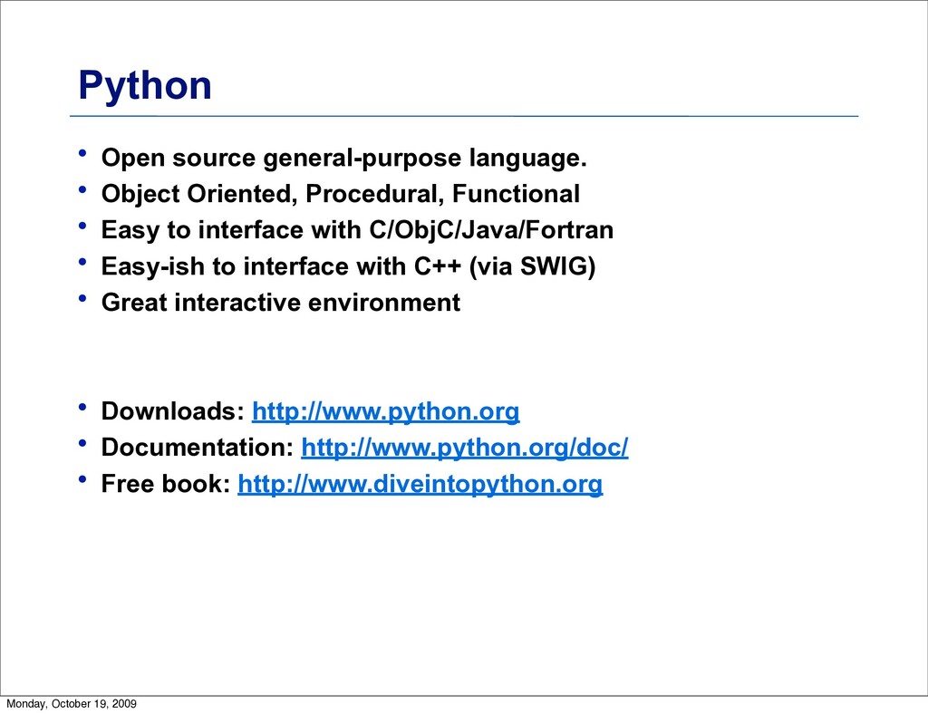
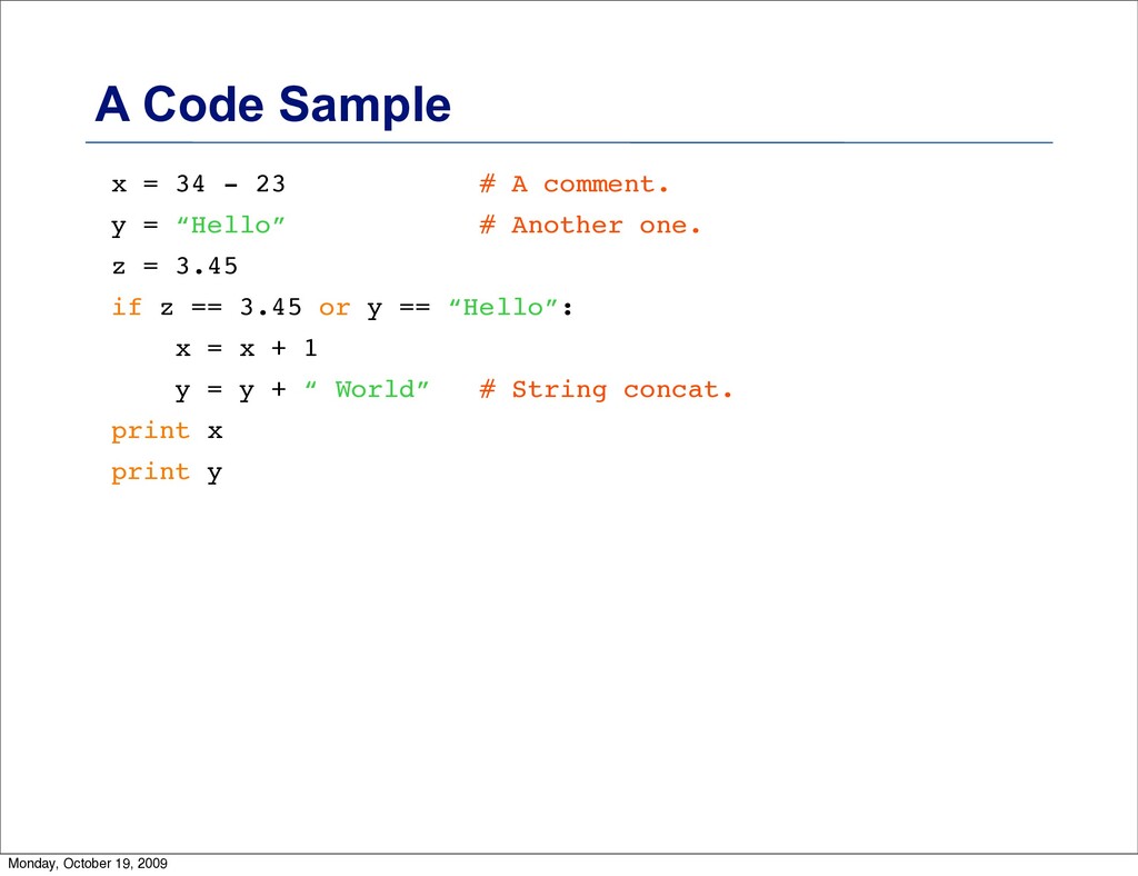
Python is an interpreted, high-level, general-purpose programming language. Created by Guido van Rossum and first released in 1991, Python's design philosophy emphasizes code readability with its notable use of significant whitespace.. For More Messages Visit us at Sharethumb

Transcript

1. Introduction to Python Heavily based on presentations by Matt Huenerfauth (Penn State) Guido van Rossum (Google) Richard P. Muller (Caltech) ... Monday, October 19, 2009
2. • Open source general-purpose language. • Object Oriented, Procedural, Functional • Easy to interface with C/ObjC/Java/Fortran • Easy-ish to interface with C++ (via SWIG) • Great interactive environment • Downloads: http://www.python.org • Documentation: http://www.python.org/doc/ • Free book: http://www.diveintopython.org Python Monday, October 19, 2009
3. 2.5.x / 2.6.x / 3.x ??? • “Current” version is 2.6.x • “Mainstream” version is 2.5.x • The new kid on the block is 3.x You probably want 2.5.x unless you are starting from scratch. Then maybe 3.x Monday, October 19, 2009
4. Technical Issues Installing & Running Python Monday, October 19, 2009
5. Binaries • Python comes pre-installed with Mac OS X and Linux. • Windows binaries from http://python.org/ • You might not have to do anything! Monday, October 19, 2009
6. The Python Interpreter • Interactive interface to Python % python Python 2.5 (r25:51908, May 25 2007, 16:14:04) [GCC 4.1.2 20061115 (prerelease) (SUSE Linux)] on linux2 Type "help", "copyright", "credits" or "license" for more information. >>> • Python interpreter evaluates inputs: >>> 3*(7+2) 27 • Python prompts with ‘>>>’. • To exit Python: • CTRL-D Monday, October 19, 2009
7. Running Programs on UNIX % python filename.py You could make the *.py file executable and add the following #!/usr/bin/env python to the top to make it runnable. Monday, October 19, 2009
8. Batteries Included • Large collection of proven modules included in the standard distribution. http://docs.python.org/modindex.html Monday, October 19, 2009
9. numpy • Offers Matlab-ish capabilities within Python • Fast array operations • 2D arrays, multi-D arrays, linear algebra etc. • Downloads: http://numpy.scipy.org/ • Tutorial: http://www.scipy.org/ Tentative_NumPy_Tutorial Monday, October 19, 2009
10. matplotlib • High quality plotting library. • Downloads: http://matplotlib.sourceforge.net/ #!/usr/bin/env python import numpy as np import matplotlib.mlab as mlab import matplotlib.pyplot as plt mu, sigma = 100, 15 x = mu + sigma*np.random.randn(10000) # the histogram of the data n, bins, patches = plt.hist(x, 50, normed=1, facecolor='green', alpha=0.75) # add a 'best fit' line y = mlab.normpdf( bins, mu, sigma) l = plt.plot(bins, y, 'r--', linewidth=1) plt.xlabel('Smarts') plt.ylabel('Probability') plt.title(r'$\mathrm{Histogram\ of\ IQ:}\ \mu=100,\ \sigma=15$') plt.axis([40, 160, 0, 0.03]) plt.grid(True) plt.show() Monday, October 19, 2009
11. PyFITS • FITS I/O made simple: • Downloads: http://www.stsci.edu/resources/ software_hardware/pyfits >>> import pyfits >>> hdulist = pyfits.open(’input.fits’) >>> hdulist.info() Filename: test1.fits No. Name Type Cards Dimensions Format 0 PRIMARY PrimaryHDU 220 () Int16 1 SCI ImageHDU 61 (800, 800) Float32 2 SCI ImageHDU 61 (800, 800) Float32 3 SCI ImageHDU 61 (800, 800) Float32 4 SCI ImageHDU 61 (800, 800) Float32 >>> hdulist[0].header[’targname’] ’NGC121’ >>> scidata = hdulist[1].data >>> scidata.shape (800, 800) >>> scidata.dtype.name ’float32’ >>> scidata[30:40,10:20] = scidata[1,4] = 999 Monday, October 19, 2009
12. pyds9 / python-sao • Interaction with DS9 • Display Python 1-D and 2-D arrays in DS9 • Display FITS files in DS9 • Downloads: Ask Eric Mandel :-) • Downloads: http://code.google.com/p/python-sao/ Monday, October 19, 2009
13. Wrappers for Astronomical Packages • CasaPy (Casa) • PYGILDAS (GILDAS) • ParselTongue (AIPS) • PyRAF (IRAF) • PyMIDAS (MIDAS) • PyIMSL (IMSL) Monday, October 19, 2009
14. Custom Distributions • Python(x,y): http://www.pythonxy.com/ • Python(x,y) is a free scientific and engineering development software for numerical computations, data analysis and data visualization • Sage: http://www.sagemath.org/ • Sage is a free open-source mathematics software system licensed under the GPL. It combines the power of many existing open-source packages into a common Python-based interface. Monday, October 19, 2009
15. Extra Astronomy Links • iPython (better shell, distributed computing): http://ipython.scipy.org/ • SciPy (collection of science tools): http:// www.scipy.org/ • Python Astronomy Modules: http:// astlib.sourceforge.net/ • Python Astronomer Wiki: http://macsingularity.org/ astrowiki/tiki-index.php?page=python • AstroPy: http://www.astro.washington.edu/users/ rowen/AstroPy.html • Python for Astronomers: http://www.iac.es/ sieinvens/siepedia/pmwiki.php? n=HOWTOs.EmpezandoPython Monday, October 19, 2009
16. The Basics Monday, October 19, 2009
17. A Code Sample x = 34 - 23 # A comment. y = “Hello” # Another one. z = 3.45 if z == 3.45 or y == “Hello”: x = x + 1 y = y + “ World” # String concat. print x print y Monday, October 19, 2009
18. Enough to Understand the Code • Assignment uses = and comparison uses ==. • For numbers + - * / % are as expected. • Special use of + for string concatenation. • Special use of % for string formatting (as with printf in C) • Logical operators are words (and, or, not) not symbols • The basic printing command is print. • The first assignment to a variable creates it. • Variable types don’t need to be declared. • Python figures out the variable types on its own. Monday, October 19, 2009
19. Basic Datatypes • Integers (default for numbers) z = 5 / 2 # Answer is 2, integer division. • Floats x = 3.456 • Strings • Can use “” or ‘’ to specify. “abc” ‘abc’ (Same thing.) • Unmatched can occur within the string. “matt’s” • Use triple double-quotes for multi-line strings or strings than contain both ‘ and “ inside of them: “““a‘b“c””” Monday, October 19, 2009
20. Whitespace Whitespace is meaningful in Python: especially indentation and placement of newlines. • Use a newline to end a line of code. • Use \ when must go to next line prematurely. • No braces { } to mark blocks of code in Python… Use consistent indentation instead. • The first line with less indentation is outside of the block. • The first line with more indentation starts a nested block • Often a colon appears at the start of a new block. (E.g. for function and class definitions.) Monday, October 19, 2009
21. Comments • Start comments with # – the rest of line is ignored. • Can include a “documentation string” as the first line of any new function or class that you define. • The development environment, debugger, and other tools use it: it’s good style to include one. def my_function(x, y): “““This is the docstring. This function does blah blah blah.””” # The code would go here... Monday, October 19, 2009
22. Assignment • Binding a variable in Python means setting a name to hold a reference to some object. • Assignment creates references, not copies • Names in Python do not have an intrinsic type. Objects have types. • Python determines the type of the reference automatically based on the data object assigned to it. • You create a name the first time it appears on the left side of an assignment expression: ! x = 3 • A reference is deleted via garbage collection after any names bound to it have passed out of scope. Monday, October 19, 2009
23. Accessing Non-Existent Names • If you try to access a name before it’s been properly created (by placing it on the left side of an assignment), you’ll get an error. >>> y Traceback (most recent call last): File "<pyshell#16>", line 1, in -toplevel- y NameError: name ‘y' is not defined >>> y = 3 >>> y 3 Monday, October 19, 2009
24. Multiple Assignment • You can also assign to multiple names at the same time. >>> x, y = 2, 3 >>> x 2 >>> y 3 Monday, October 19, 2009
25. Naming Rules • Names are case sensitive and cannot start with a number. They can contain letters, numbers, and underscores. bob Bob _bob _2_bob_ bob_2 BoB • There are some reserved words: and, assert, break, class, continue, def, del, elif, else, except, exec, finally, for, from, global, if, import, in, is, lambda, not, or, pass, print, raise, return, try, while Monday, October 19, 2009
26. Understanding Reference Semantics in Python Monday, October 19, 2009
27. Understanding Reference Semantics • Assignment manipulates references —x = y does not make a copy of the object y references —x = y makes x reference the object y references • Very useful; but beware! • Example: >>> a = [1, 2, 3] # a now references the list [1, 2, 3] >>> b = a # b now references what a references >>> a.append(4) # this changes the list a references >>> print b # if we print what b references, [1, 2, 3, 4] # SURPRISE! It has changed… Why?? Monday, October 19, 2009
28. Understanding Reference Semantics II • There is a lot going on when we type: x = 3 • First, an integer 3 is created and stored in memory • A name x is created • An reference to the memory location storing the 3 is then assigned to the name x • So: When we say that the value of x is 3 • we mean that x now refers to the integer 3 Type: Integer Data: 3 Name: x Ref: <address1> name list memory Monday, October 19, 2009
29. Understanding Reference Semantics III • The data 3 we created is of type integer. In Python, the datatypes integer, float, and string (and tuple) are “immutable.” • This doesn’t mean we can’t change the value of x, i.e. change what x refers to … • For example, we could increment x: >>> x = 3 >>> x = x + 1 >>> print x 4 Monday, October 19, 2009
30. Understanding Reference Semantics IV • If we increment x, then what’s really happening is: 1. The reference of name x is looked up. 2. The value at that reference is retrieved. Type: Integer Data: 3 Name: x Ref: <address1> >>> x = x + 1 Monday, October 19, 2009
31. Understanding Reference Semantics IV • If we increment x, then what’s really happening is: 1. The reference of name x is looked up. 2. The value at that reference is retrieved. 3. The 3+1 calculation occurs, producing a new data element 4 which is assigned to a fresh memory location with a new reference. Type: Integer Data: 3 Name: x Ref: <address1> Type: Integer Data: 4 >>> x = x + 1 Monday, October 19, 2009
32. Understanding Reference Semantics IV • If we increment x, then what’s really happening is: 1. The reference of name x is looked up. 2. The value at that reference is retrieved. 3. The 3+1 calculation occurs, producing a new data element 4 which is assigned to a fresh memory location with a new reference. 4. The name x is changed to point to this new reference. Type: Integer Data: 3 Name: x Ref: <address1> Type: Integer Data: 4 >>> x = x + 1 Monday, October 19, 2009
33. Understanding Reference Semantics IV • If we increment x, then what’s really happening is: 1. The reference of name x is looked up. 2. The value at that reference is retrieved. 3. The 3+1 calculation occurs, producing a new data element 4 which is assigned to a fresh memory location with a new reference. 4. The name x is changed to point to this new reference. 5. The old data 3 is garbage collected if no name still refers to it. Name: x Ref: <address1> Type: Integer Data: 4 >>> x = x + 1 Monday, October 19, 2009
34. Assignment 1 • So, for simple built-in datatypes (integers, floats, strings), assignment behaves as you would expect: >>> x = 3 # Creates 3, name x refers to 3 >>> y = x # Creates name y, refers to 3. >>> y = 4 # Creates ref for 4. Changes y. >>> print x # No effect on x, still ref 3. 3 Monday, October 19, 2009
35. Assignment 1 • So, for simple built-in datatypes (integers, floats, strings), assignment behaves as you would expect: >>> x = 3 # Creates 3, name x refers to 3 >>> y = x # Creates name y, refers to 3. >>> y = 4 # Creates ref for 4. Changes y. >>> print x # No effect on x, still ref 3. 3 Type: Integer Data: 3 Name: x Ref: <address1> Monday, October 19, 2009
36. Assignment 1 • So, for simple built-in datatypes (integers, floats, strings), assignment behaves as you would expect: >>> x = 3 # Creates 3, name x refers to 3 >>> y = x # Creates name y, refers to 3. >>> y = 4 # Creates ref for 4. Changes y. >>> print x # No effect on x, still ref 3. 3 Type: Integer Data: 3 Name: x Ref: <address1> Name: y Ref: <address1> Monday, October 19, 2009
37. Assignment 1 • So, for simple built-in datatypes (integers, floats, strings), assignment behaves as you would expect: >>> x = 3 # Creates 3, name x refers to 3 >>> y = x # Creates name y, refers to 3. >>> y = 4 # Creates ref for 4. Changes y. >>> print x # No effect on x, still ref 3. 3 Type: Integer Data: 3 Name: x Ref: <address1> Type: Integer Data: 4 Name: y Ref: <address1> Monday, October 19, 2009
38. Assignment 1 • So, for simple built-in datatypes (integers, floats, strings), assignment behaves as you would expect: >>> x = 3 # Creates 3, name x refers to 3 >>> y = x # Creates name y, refers to 3. >>> y = 4 # Creates ref for 4. Changes y. >>> print x # No effect on x, still ref 3. 3 Type: Integer Data: 3 Name: x Ref: <address1> Type: Integer Data: 4 Name: y Ref: <address2> Monday, October 19, 2009
39. Assignment 1 • So, for simple built-in datatypes (integers, floats, strings), assignment behaves as you would expect: >>> x = 3 # Creates 3, name x refers to 3 >>> y = x # Creates name y, refers to 3. >>> y = 4 # Creates ref for 4. Changes y. >>> print x # No effect on x, still ref 3. 3 Type: Integer Data: 3 Name: x Ref: <address1> Type: Integer Data: 4 Name: y Ref: <address2> Monday, October 19, 2009
40. Assignment 2 • For other data types (lists, dictionaries, user-defined types), assignment works differently. • These datatypes are “mutable.” • When we change these data, we do it in place. • We don’t copy them into a new memory address each time. • If we type y=x and then modify y, both x and y are changed. >>> x = 3 x = some mutable object >>> y = x y = x >>> y = 4 make a change to y >>> print x look at x 3 x will be changed as well immutable mutable Monday, October 19, 2009
41. a 1 2 3 b a 1 2 3 b 4 a = [1, 2, 3] a.append(4) b = a a 1 2 3 Why? Changing a Shared List Monday, October 19, 2009
42. Our surprising example surprising no more... • So now, here’s our code: >>> a = [1, 2, 3] # a now references the list [1, 2, 3] >>> b = a # b now references what a references >>> a.append(4) # this changes the list a references >>> print b # if we print what b references, [1, 2, 3, 4] # SURPRISE! It has changed… Monday, October 19, 2009
43. Sequence types: Tuples, Lists, and Strings Monday, October 19, 2009
44. Sequence Types 1. Tuple • A simple immutable ordered sequence of items • Items can be of mixed types, including collection types 2. Strings • Immutable • Conceptually very much like a tuple 3. List • Mutable ordered sequence of items of mixed types Monday, October 19, 2009
45. Similar Syntax • All three sequence types (tuples, strings, and lists) share much of the same syntax and functionality. • Key difference: • Tuples and strings are immutable • Lists are mutable • The operations shown in this section can be applied to all sequence types • most examples will just show the operation performed on one Monday, October 19, 2009
46. Sequence Types 1 • Tuples are defined using parentheses (and commas). >>> tu = (23, ‘abc’, 4.56, (2,3), ‘def’) • Lists are defined using square brackets (and commas). >>> li = [“abc”, 34, 4.34, 23] • Strings are defined using quotes (“, ‘, or “““). >>> st = “Hello World” >>> st = ‘Hello World’ >>> st = “““This is a multi-line string that uses triple quotes.””” Monday, October 19, 2009
47. Sequence Types 2 • We can access individual members of a tuple, list, or string using square bracket “array” notation. • Note that all are 0 based… >>> tu = (23, ‘abc’, 4.56, (2,3), ‘def’) >>> tu[1] # Second item in the tuple. ‘abc’ >>> li = [“abc”, 34, 4.34, 23] >>> li[1] # Second item in the list. 34 >>> st = “Hello World” >>> st[1] # Second character in string. ‘e’ Monday, October 19, 2009
48. Positive and negative indices >>> t = (23, ‘abc’, 4.56, (2,3), ‘def’) Positive index: count from the left, starting with 0. >>> t[1] ‘abc’ Negative lookup: count from right, starting with –1. >>> t[-3] 4.56 Monday, October 19, 2009
49. Slicing: Return Copy of a Subset 1 >>> t = (23, ‘abc’, 4.56, (2,3), ‘def’) Return a copy of the container with a subset of the original members. Start copying at the first index, and stop copying before the second index. >>> t[1:4] (‘abc’, 4.56, (2,3)) You can also use negative indices when slicing. >>> t[1:-1] (‘abc’, 4.56, (2,3)) Monday, October 19, 2009
50. Slicing: Return Copy of a Subset 2 >>> t = (23, ‘abc’, 4.56, (2,3), ‘def’) Omit the first index to make a copy starting from the beginning of the container. >>> t[:2] (23, ‘abc’) Omit the second index to make a copy starting at the first index and going to the end of the container. >>> t[2:] (4.56, (2,3), ‘def’) Monday, October 19, 2009
51. Copying the Whole Sequence To make a copy of an entire sequence, you can use [:]. >>> t[:] (23, ‘abc’, 4.56, (2,3), ‘def’) Note the difference between these two lines for mutable sequences: >>> list2 = list1 # 2 names refer to 1 ref # Changing one affects both >>> list2 = list1[:] # Two independent copies, two refs Monday, October 19, 2009
52. The ‘in’ Operator • Boolean test whether a value is inside a container: >>> t = [1, 2, 4, 5] >>> 3 in t False >>> 4 in t True >>> 4 not in t False • For strings, tests for substrings >>> a = 'abcde' >>> 'c' in a True >>> 'cd' in a True >>> 'ac' in a False • Be careful: the in keyword is also used in the syntax of for loops and list comprehensions. Monday, October 19, 2009
53. The + Operator • The + operator produces a new tuple, list, or string whose value is the concatenation of its arguments. >>> (1, 2, 3) + (4, 5, 6) (1, 2, 3, 4, 5, 6) >>> [1, 2, 3] + [4, 5, 6] [1, 2, 3, 4, 5, 6] >>> “Hello” + “ ” + “World” ‘Hello World’ Monday, October 19, 2009
54. The * Operator • The * operator produces a new tuple, list, or string that “repeats” the original content. >>> (1, 2, 3) * 3 (1, 2, 3, 1, 2, 3, 1, 2, 3) >>> [1, 2, 3] * 3 [1, 2, 3, 1, 2, 3, 1, 2, 3] >>> “Hello” * 3 ‘HelloHelloHello’ Monday, October 19, 2009
55. Mutability: Tuples vs. Lists Monday, October 19, 2009
56. Tuples: Immutable >>> t = (23, ‘abc’, 4.56, (2,3), ‘def’) >>> t[2] = 3.14 Traceback (most recent call last): File "<pyshell#75>", line 1, in -toplevel- tu[2] = 3.14 TypeError: object doesn't support item assignment You can’t change a tuple. You can make a fresh tuple and assign its reference to a previously used name. >>> t = (23, ‘abc’, 3.14, (2,3), ‘def’) Monday, October 19, 2009
57. Lists: Mutable >>> li = [‘abc’, 23, 4.34, 23] >>> li[1] = 45 >>> li [‘abc’, 45, 4.34, 23] • We can change lists in place. • Name li still points to the same memory reference when we’re done. • The mutability of lists means that they aren’t as fast as tuples. Monday, October 19, 2009
58. Operations on Lists Only 1 >>> li = [1, 11, 3, 4, 5] >>> li.append(‘a’) # Our first exposure to method syntax >>> li [1, 11, 3, 4, 5, ‘a’] >>> li.insert(2, ‘i’) >>>li [1, 11, ‘i’, 3, 4, 5, ‘a’] Monday, October 19, 2009
59. The extend method vs the + operator. • + creates a fresh list (with a new memory reference) • extend operates on list li in place. >>> li.extend([9, 8, 7]) >>>li [1, 2, ‘i’, 3, 4, 5, ‘a’, 9, 8, 7] Confusing: • Extend takes a list as an argument. • Append takes a singleton as an argument. >>> li.append([10, 11, 12]) >>> li [1, 2, ‘i’, 3, 4, 5, ‘a’, 9, 8, 7, [10, 11, 12]] Monday, October 19, 2009
60. Operations on Lists Only 3 >>> li = [‘a’, ‘b’, ‘c’, ‘b’] >>> li.index(‘b’) # index of first occurrence 1 >>> li.count(‘b’) # number of occurrences 2 >>> li.remove(‘b’) # remove first occurrence >>> li [‘a’, ‘c’, ‘b’] Monday, October 19, 2009
61. Operations on Lists Only 4 >>> li = [5, 2, 6, 8] >>> li.reverse() # reverse the list *in place* >>> li [8, 6, 2, 5] >>> li.sort() # sort the list *in place* >>> li [2, 5, 6, 8] >>> li.sort(some_function) # sort in place using user-defined comparison Monday, October 19, 2009
62. Tuples vs. Lists • Lists slower but more powerful than tuples. • Lists can be modified, and they have lots of handy operations we can perform on them. • Tuples are immutable and have fewer features. • To convert between tuples and lists use the list() and tuple() functions: li = list(tu) tu = tuple(li) Monday, October 19, 2009
63. Dictionaries 63 Monday, October 19, 2009
64. Dictionaries: A Mapping type • Dictionaries store a mapping between a set of keys and a set of values. • Keys can be any immutable type. • Values can be any type • A single dictionary can store values of different types • You can define, modify, view, lookup, and delete the key-value pairs in the dictionary. Monday, October 19, 2009
65. Using dictionaries >>> d = {‘user’:‘bozo’, ‘pswd’:1234} >>> d[‘user’] ‘bozo’ >>> d[‘pswd’] 1234 >>> d[‘bozo’] Traceback (innermost last): File ‘<interactive input>’ line 1, in ? KeyError: bozo >>> d = {‘user’:‘bozo’, ‘pswd’:1234} >>> d[‘user’] = ‘clown’ >>> d {‘user’:‘clown’, ‘pswd’:1234} >>> d[‘id’] = 45 >>> d {‘user’:‘clown’, ‘id’:45, ‘pswd’:1234} >>> d = {‘user’:‘bozo’, ‘p’:1234, ‘i’:34} >>> del d[‘user’] # Remove one. >>> d {‘p’:1234, ‘i’:34} >>> d.clear() # Remove all. >>> d {} >>> d = {‘user’:‘bozo’, ‘p’:1234, ‘i’:34} >>> d.keys() # List of keys. [‘user’, ‘p’, ‘i’] >>> d.values() # List of values. [‘bozo’, 1234, 34] >>> d.items() # List of item tuples. [(‘user’,‘bozo’), (‘p’,1234), (‘i’,34)] Monday, October 19, 2009
66. Functions Monday, October 19, 2009
67. Functions • def creates a function and assigns it a name • return sends a result back to the caller • Arguments are passed by assignment • Arguments and return types are not declared def <name>(arg1, arg2, ..., argN): ! <statements> ! return <value> def times(x,y): ! return x*y Monday, October 19, 2009
68. Passing Arguments to Functions • Arguments are passed by assignment • Passed arguments are assigned to local names • Assignment to argument names don't affect the caller • Changing a mutable argument may affect the caller def changer (x,y): ! x = 2! ! ! # changes local value of x only ! y[0] = 'hi'! ! # changes shared object Monday, October 19, 2009
69. Optional Arguments • Can define defaults for arguments that need not be passed def func(a, b, c=10, d=100): ! print a, b, c, d >>> func(1,2) 1 2 10 100 >>> func(1,2,3,4) 1,2,3,4 Monday, October 19, 2009
70. Gotchas • All functions in Python have a return value • even if no return line inside the code. • Functions without a return return the special value None. • There is no function overloading in Python. • Two different functions can’t have the same name, even if they have different arguments. • Functions can be used as any other data type. They can be: • Arguments to function • Return values of functions • Assigned to variables • Parts of tuples, lists, etc Monday, October 19, 2009
71. Control of Flow 71 Monday, October 19, 2009
72. Examples if x == 3: print “X equals 3.” elif x == 2: print “X equals 2.” else: print “X equals something else.” print “This is outside the ‘if’.” x = 3 while x < 10: if x > 7: x += 2 continue x = x + 1 print “Still in the loop.” if x == 8: break print “Outside of the loop.” assert(number_of_players < 5) for x in range(10): if x > 7: x += 2 continue x = x + 1 print “Still in the loop.” if x == 8: break print “Outside of the loop.” Monday, October 19, 2009
73. Modules Monday, October 19, 2009
74. Why Use Modules? • Code reuse • Routines can be called multiple times within a program • Routines can be used from multiple programs • Namespace partitioning • Group data together with functions used for that data • Implementing shared services or data • Can provide global data structure that is accessed by multiple subprograms Monday, October 19, 2009
75. Modules • Modules are functions and variables defined in separate files • Items are imported using from or import from module import function function() import module module.function() • Modules are namespaces • Can be used to organize variable names, i.e. atom.position = atom.position - molecule.position Monday, October 19, 2009
76. Classes and Objects Monday, October 19, 2009
77. What is an Object? • A software item that contains variables and methods • Object Oriented Design focuses on • Encapsulation: —dividing the code into a public interface, and a private implementation of that interface • Polymorphism: —the ability to overload standard operators so that they have appropriate behavior based on their context • Inheritance: —the ability to create subclasses that contain specializations of their parents Monday, October 19, 2009
78. Example class atom(object): ! def __init__(self,atno,x,y,z): ! ! self.atno = atno ! ! self.position = (x,y,z) ! def symbol(self): # a class method ! ! return Atno_to_Symbol[atno] ! def __repr__(self): # overloads printing ! ! return '%d %10.4f %10.4f %10.4f' % ! ! ! (self.atno, self.position[0], ! ! ! self.position[1],self.position[2]) >>> at = atom(6,0.0,1.0,2.0) >>> print at 6 0.0000 1.0000 2.0000 >>> at.symbol() 'C' Monday, October 19, 2009
79. Atom Class • Overloaded the default constructor • Defined class variables (atno,position) that are persistent and local to the atom object • Good way to manage shared memory: • instead of passing long lists of arguments, encapsulate some of this data into an object, and pass the object. • much cleaner programs result • Overloaded the print operator • We now want to use the atom class to build molecules... Monday, October 19, 2009
80. Molecule Class class molecule: ! def __init__(self,name='Generic'): ! ! self.name = name ! ! self.atomlist = [] ! def addatom(self,atom): ! ! self.atomlist.append(atom) ! def __repr__(self): ! ! str = 'This is a molecule named %s\n' % self.name ! ! str = str+'It has %d atoms\n' % len(self.atomlist) ! ! for atom in self.atomlist: ! ! ! str = str + `atom` + '\n' ! ! return str Monday, October 19, 2009
81. Using Molecule Class >>> mol = molecule('Water') >>> at = atom(8,0.,0.,0.) >>> mol.addatom(at) >>> mol.addatom(atom(1,0.,0.,1.)) >>> mol.addatom(atom(1,0.,1.,0.)) >>> print mol This is a molecule named Water It has 3 atoms 8 0.000 0.000 0.000 1 0.000 0.000 1.000 1 0.000 1.000 0.000 • Note that the print function calls the atoms print function • Code reuse: only have to type the code that prints an atom once; this means that if you change the atom specification, you only have one place to update. Monday, October 19, 2009
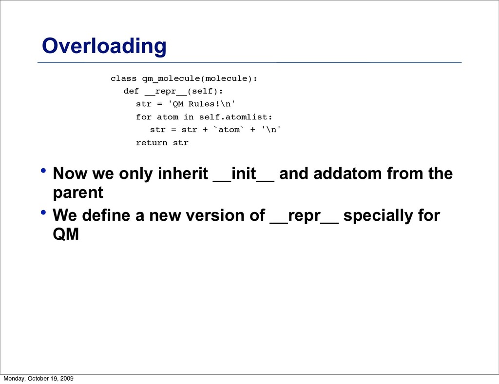
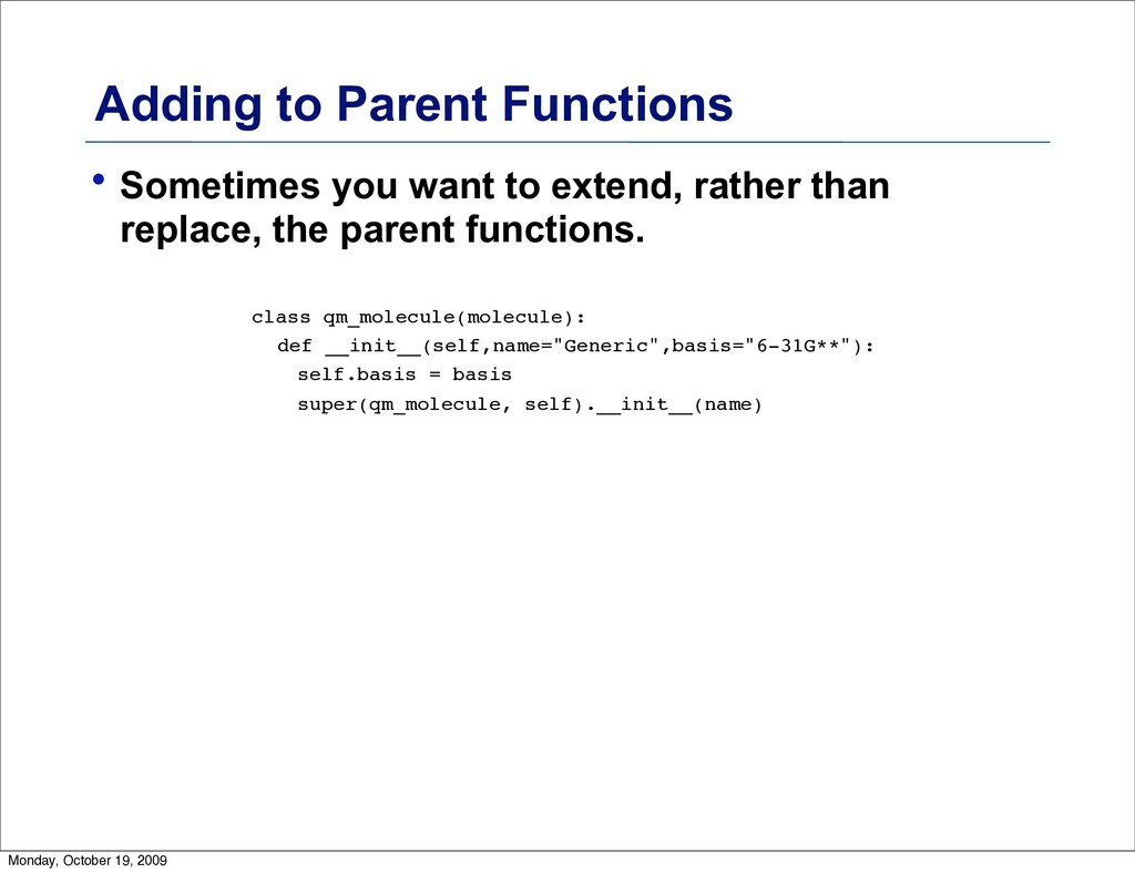
82. Inheritance class qm_molecule(molecule): def addbasis(self): self.basis = [] for atom in self.atomlist: self.basis = add_bf(atom,self.basis) • __init__, __repr__, and __addatom__ are taken from the parent class (molecule) • Added a new function addbasis() to add a basis set • Another example of code reuse • Basic functions don't have to be retyped, just inherited • Less to rewrite when specifications change Monday, October 19, 2009
83. Overloading class qm_molecule(molecule): def __repr__(self): ! ! str = 'QM Rules!\n' ! ! for atom in self.atomlist: ! ! ! str = str + `atom` + '\n' ! ! return str • Now we only inherit __init__ and addatom from the parent • We define a new version of __repr__ specially for QM Monday, October 19, 2009
84. Adding to Parent Functions • Sometimes you want to extend, rather than replace, the parent functions. class qm_molecule(molecule): ! def __init__(self,name="Generic",basis="6-31G**"): ! ! self.basis = basis ! ! super(qm_molecule, self).__init__(name) Monday, October 19, 2009
85. Public and Private Data • In Python anything with two leading underscores is private __a, __my_variable • Anything with one leading underscore is semi- private, and you should feel guilty accessing this data directly. _b • Sometimes useful as an intermediate step to making data private Monday, October 19, 2009
86. The Extra Stuff... 86 Monday, October 19, 2009
87. File I/O, Strings, Exceptions... fileptr = open(‘filename’) somestring = fileptr.read() for line in fileptr: print line fileptr.close() >>> a = 1 >>> b = 2.4 >>> c = 'Tom' >>> '%s has %d coins worth a total of $%.02f' % (c, a, b) 'Tom has 1 coins worth a total of $2.40' >>> try: ... 1 / 0 ... except: ... print('That was silly!') ... finally: ... print('This gets executed no matter what') ... That was silly! This gets executed no matter what Monday, October 19, 2009