Technology. Government sponsorship acknowledged Stephen R. Taylor Astrophysical Inference Of Supermassive Black-hole Binaries With Pulsar-timing Arrays JET PROPULSION LABORATORY, CALIFORNIA INSTITUTE OF TECHNOLOGY
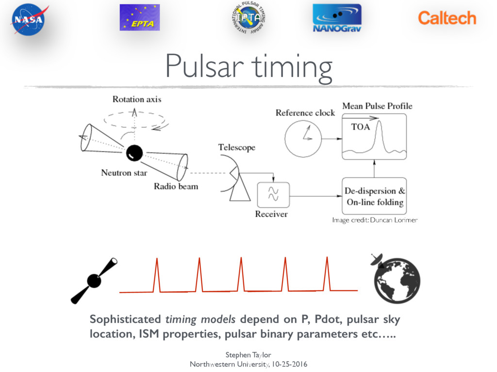
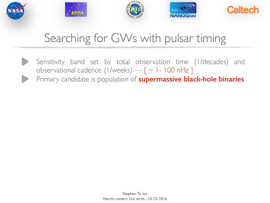
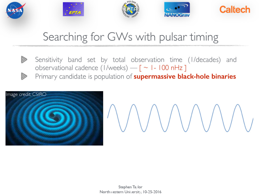
observation time (1/decades) and observational cadence (1/weeks) — [ ~ 1- 100 nHz ] Primary candidate is population of supermassive black-hole binaries Searching for GWs with pulsar timing
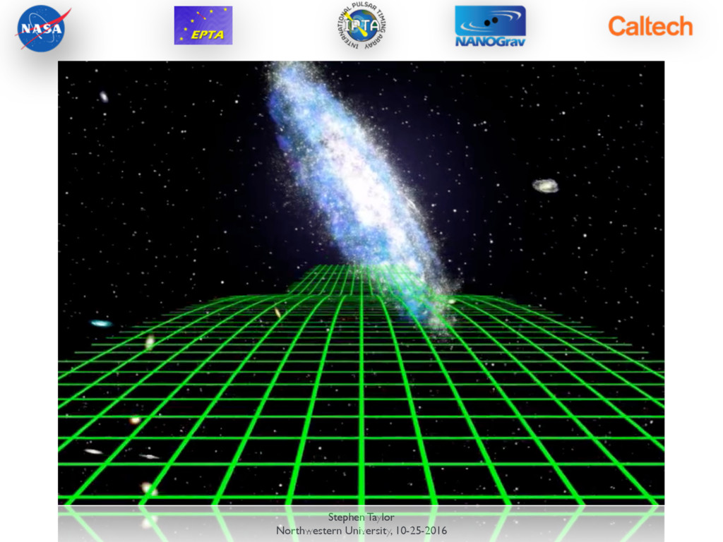
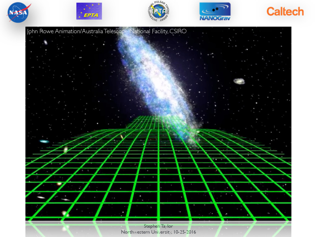
observation time (1/decades) and observational cadence (1/weeks) — [ ~ 1- 100 nHz ] Primary candidate is population of supermassive black-hole binaries Image credit: CSIRO Searching for GWs with pulsar timing
observation time (1/decades) and observational cadence (1/weeks) — [ ~ 1- 100 nHz ] Primary candidate is population of supermassive black-hole binaries Image credit: CSIRO Searching for GWs with pulsar timing
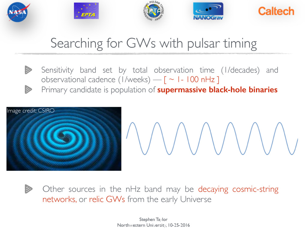
observation time (1/decades) and observational cadence (1/weeks) — [ ~ 1- 100 nHz ] Primary candidate is population of supermassive black-hole binaries Other sources in the nHz band may be decaying cosmic-string networks, or relic GWs from the early Universe Image credit: CSIRO Searching for GWs with pulsar timing
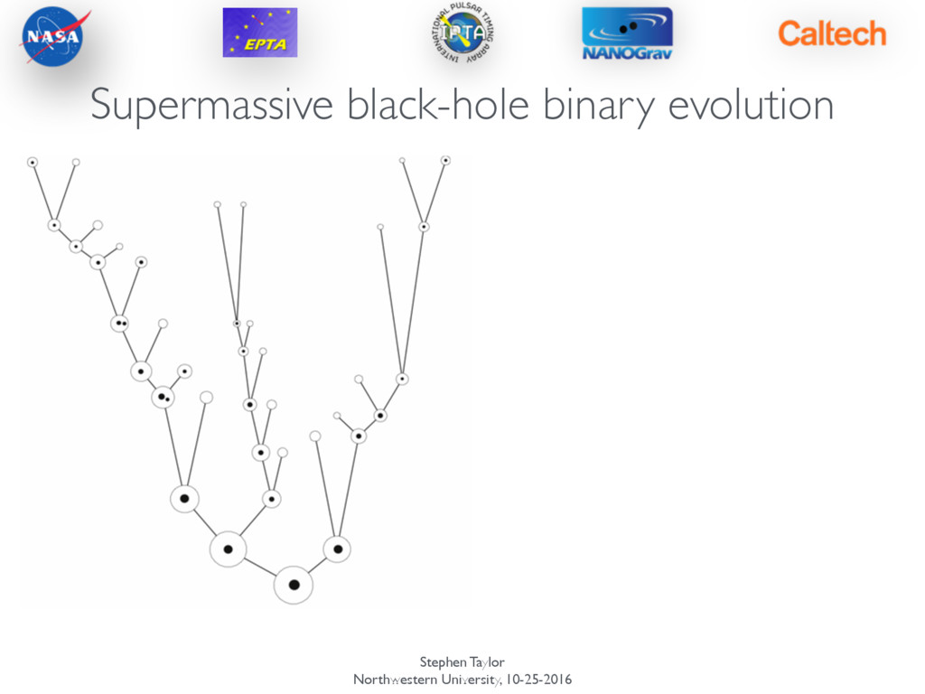
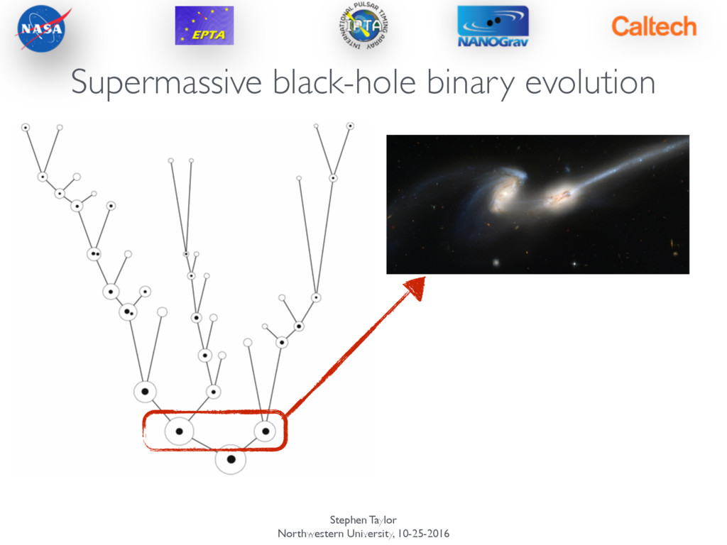
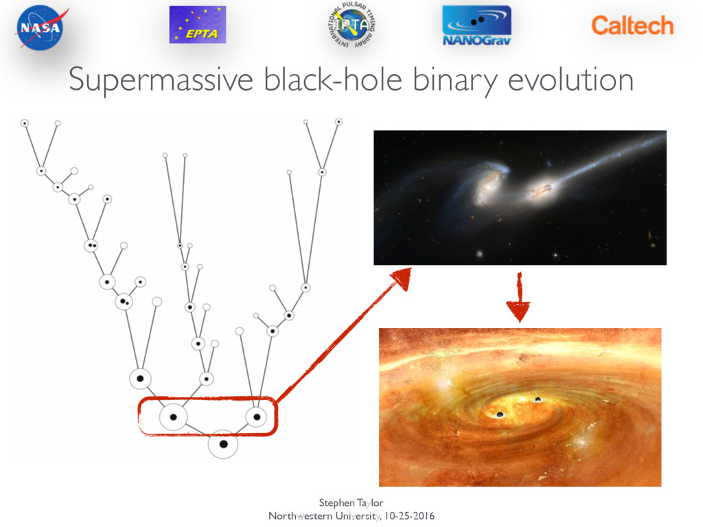
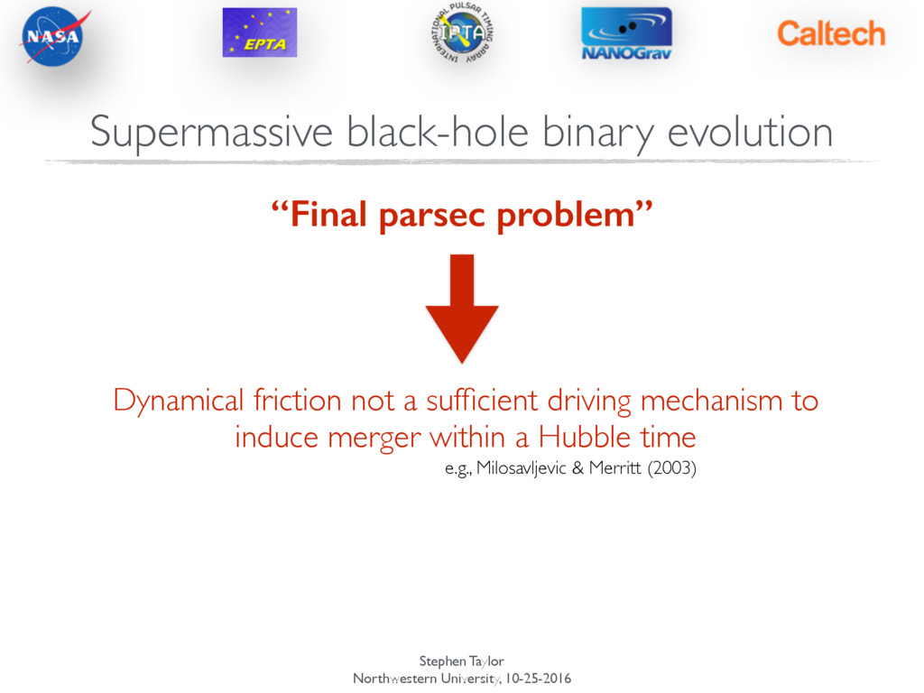
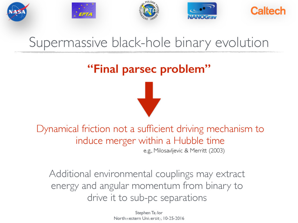
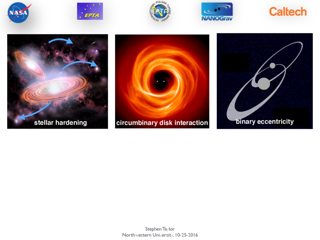
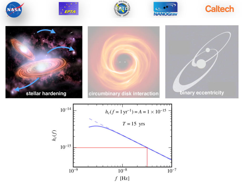
not a sufficient driving mechanism to induce merger within a Hubble time e.g., Milosavljevic & Merritt (2003) Additional environmental couplings may extract energy and angular momentum from binary to drive it to sub-pc separations Supermassive black-hole binary evolution
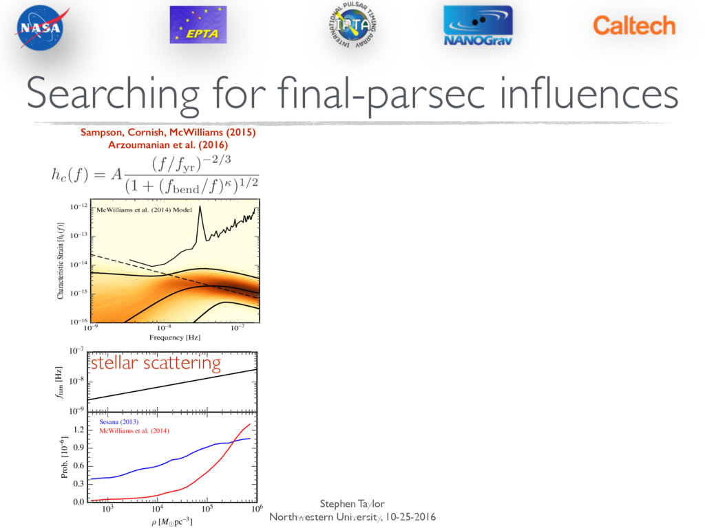
10-9 10-8 10-7 Frequency [Hz] 10-16 10-15 10-14 10-13 10-12 Characteristic Strain [hc(f)] McWilliams et al. (2014) Model Figure 5. Probability density plots of the recovered GWB spectra for models A and B using the broken-power-law model parameterized by (Agw, fbend, and ) as discussed in the text. The thick black lines indicate the 95% credible region and median of the GWB spectrum. The dashed line shows the 95% upper limit on the amplitude of purely GW-driven spectrum using the Gaussian priors on the amplitude from models A and B, respectively. The thin black curve shows the 95% upper limit on the GWB spectrum from the spectral analysis. 16 10-9 10-8 10-7 fturn [Hz] 103 104 105 106 ⇢ [M pc-3] 0.0 0.3 0.6 0.9 1.2 Prob. [10-6] Sesana (2013) McWilliams et al. (2014) stellar scattering hc(f) = A (f/fyr) 2/3 (1 + (fbend/f))1/2 Sampson, Cornish, McWilliams (2015) Arzoumanian et al. (2016)
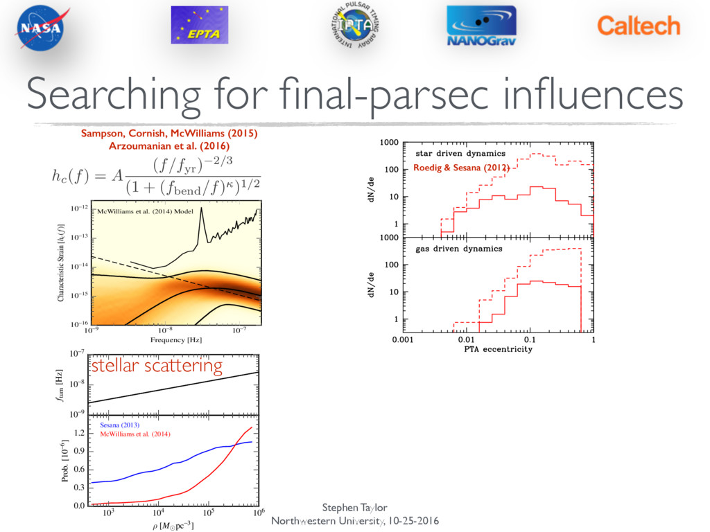
10-9 10-8 10-7 Frequency [Hz] 10-16 10-15 10-14 10-13 10-12 Characteristic Strain [hc(f)] McWilliams et al. (2014) Model Figure 5. Probability density plots of the recovered GWB spectra for models A and B using the broken-power-law model parameterized by (Agw, fbend, and ) as discussed in the text. The thick black lines indicate the 95% credible region and median of the GWB spectrum. The dashed line shows the 95% upper limit on the amplitude of purely GW-driven spectrum using the Gaussian priors on the amplitude from models A and B, respectively. The thin black curve shows the 95% upper limit on the GWB spectrum from the spectral analysis. 16 10-9 10-8 10-7 fturn [Hz] 103 104 105 106 ⇢ [M pc-3] 0.0 0.3 0.6 0.9 1.2 Prob. [10-6] Sesana (2013) McWilliams et al. (2014) stellar scattering hc(f) = A (f/fyr) 2/3 (1 + (fbend/f))1/2 Figure 2. Eccentricity population of MBHBs detectable by ELISA/NGO and PTAs, expected in stellar and gaseous environments. Left panel: The solid histograms represent the efficient models whereas the dashed histograms are for the inefficient models. Right panel: solid his- tograms include all sources producing timing residuals above 3 ns, dashed histograms include all sources producing residual above 10 ns. mechanism (gas/star) we consider two scenarios (efficient/inefficient), to give an idea of the expected eccentricity range. The models are the following (i) gas-efficient: α = 0.3, ˙ m = 1. The migration timescale is maximized for this high values of the disc parameters, and the decoupling occurs in the very late stage of the MBHB evolution; Roedig & Sesana (2012) Sampson, Cornish, McWilliams (2015) Arzoumanian et al. (2016)
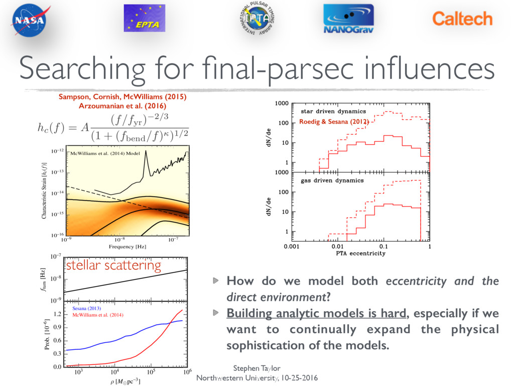
10-9 10-8 10-7 Frequency [Hz] 10-16 10-15 10-14 10-13 10-12 Characteristic Strain [hc(f)] McWilliams et al. (2014) Model Figure 5. Probability density plots of the recovered GWB spectra for models A and B using the broken-power-law model parameterized by (Agw, fbend, and ) as discussed in the text. The thick black lines indicate the 95% credible region and median of the GWB spectrum. The dashed line shows the 95% upper limit on the amplitude of purely GW-driven spectrum using the Gaussian priors on the amplitude from models A and B, respectively. The thin black curve shows the 95% upper limit on the GWB spectrum from the spectral analysis. 16 10-9 10-8 10-7 fturn [Hz] 103 104 105 106 ⇢ [M pc-3] 0.0 0.3 0.6 0.9 1.2 Prob. [10-6] Sesana (2013) McWilliams et al. (2014) stellar scattering hc(f) = A (f/fyr) 2/3 (1 + (fbend/f))1/2 Figure 2. Eccentricity population of MBHBs detectable by ELISA/NGO and PTAs, expected in stellar and gaseous environments. Left panel: The solid histograms represent the efficient models whereas the dashed histograms are for the inefficient models. Right panel: solid his- tograms include all sources producing timing residuals above 3 ns, dashed histograms include all sources producing residual above 10 ns. mechanism (gas/star) we consider two scenarios (efficient/inefficient), to give an idea of the expected eccentricity range. The models are the following (i) gas-efficient: α = 0.3, ˙ m = 1. The migration timescale is maximized for this high values of the disc parameters, and the decoupling occurs in the very late stage of the MBHB evolution; Roedig & Sesana (2012) Sampson, Cornish, McWilliams (2015) Arzoumanian et al. (2016) How do we model both eccentricity and the direct environment? Building analytic models is hard, especially if we want to continually expand the physical sophistication of the models.
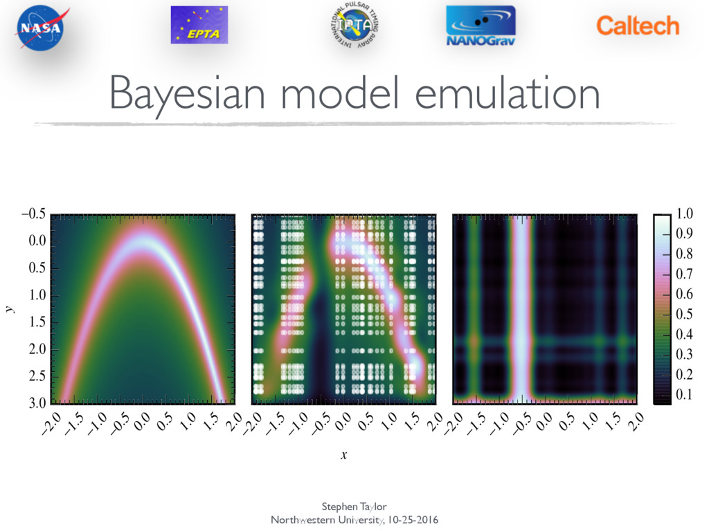
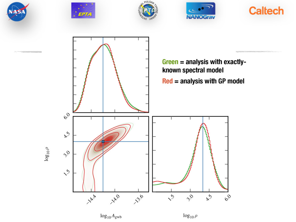
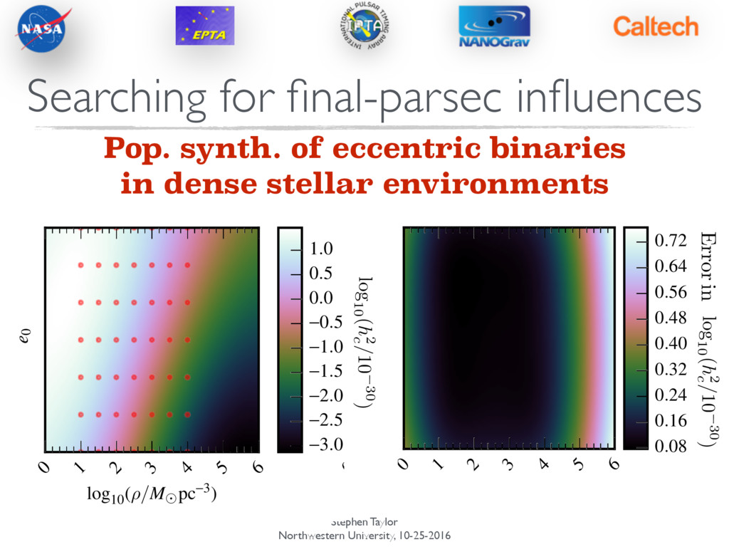
small number of expensive SMBHB population simulations. •Train a Gaussian process to learn the shape of the spectrum at different physical parameter values. •Learn the spectral variance due to finiteness of the SMBHB population. ! •We have a predictor for the shape of the spectrum, AND a measure of the uncertainty from the interpolation scheme. Searching for final-parsec influences
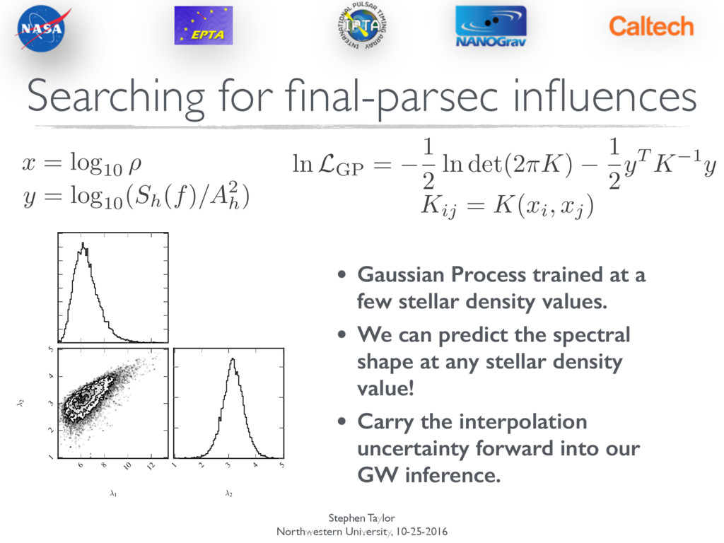
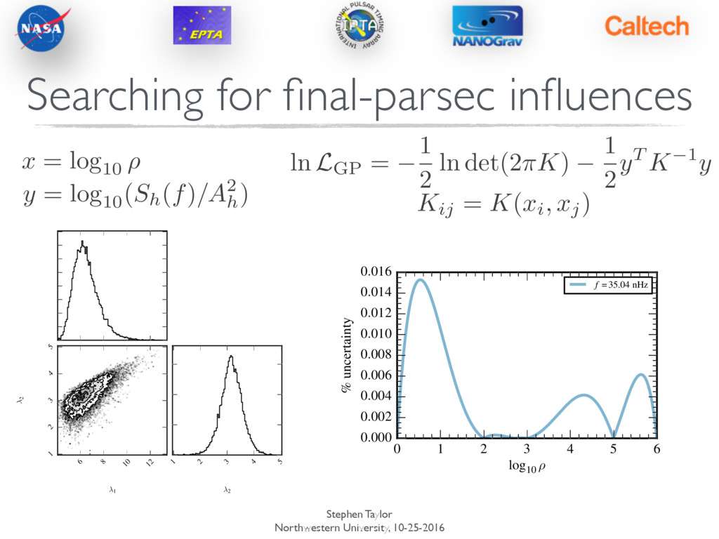
a few stellar density values. • We can predict the spectral shape at any stellar density value! • Carry the interpolation uncertainty forward into our GW inference. 6 8 10 12 1 1 2 3 4 5 2 1 2 3 4 5 2 x = log10 ⇢ y = log10( Sh( f ) /A2 h) ln LGP = 1 2 ln det(2⇡K) 1 2 yT K 1y Kij = K ( xi, xj) Searching for final-parsec influences
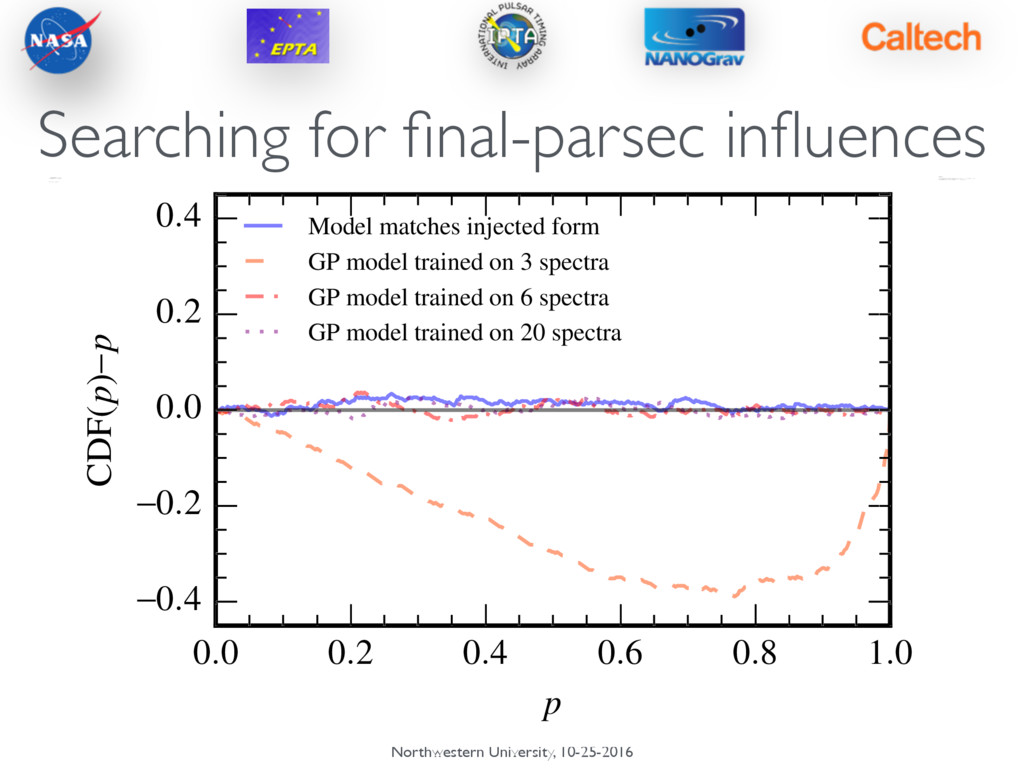
1.0 p -0.4 -0.2 0.0 0.2 0.4 CDF(p)-p Model matches injected form GP model trained on 3 spectra GP model trained on 6 spectra GP model trained on 20 spectra Searching for final-parsec influences
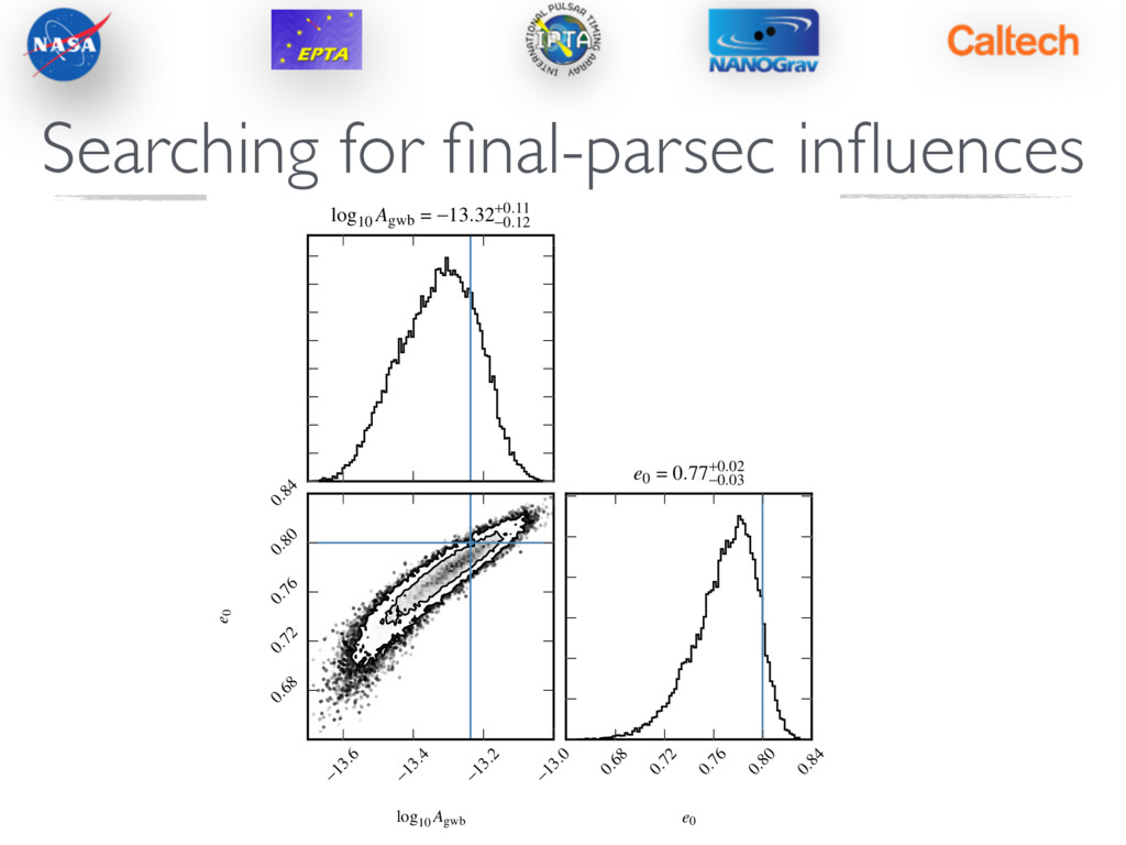
nHz gravitational-waves within a decade. [Taylor et al., ApJL, 819, L6, (2016) ] ! The strain spectrum of nHz gravitational-waves encodes the physics of the final parsec of SMBHB evolution. ! We can build physically-sophisticated spectral models by training Gaussian Processes on populations of binaries. Sometimes its easier to simulate the Universe than write down an equation. [with Laura Sampson and Joseph Simon, in prep.]
![Stephen Taylor Northwestern University, 10-25-2016 10-8 10-7 f [Hz] 10-1](https://files.speakerdeck.com/presentations/c476b02834324d1d9c4d5fb3c27a70f6/slide_30.jpg)
![Stephen Taylor Northwestern University, 10-25-2016 10-8 10-7 f [Hz] 10-1](https://files.speakerdeck.com/presentations/c476b02834324d1d9c4d5fb3c27a70f6/slide_31.jpg)
![Stephen Taylor Northwestern University, 10-25-2016 10-8 10-7 f [Hz] 10-17](https://files.speakerdeck.com/presentations/c476b02834324d1d9c4d5fb3c27a70f6/slide_36.jpg)