Institute of Technology. Government sponsorship acknowledged Stephen Taylor Supermassive Black-hole Binary Astrophysics With Pulsar-timing Arrays JET PROPULSION LABORATORY, CALIFORNIA INSTITUTE OF TECHNOLOGY
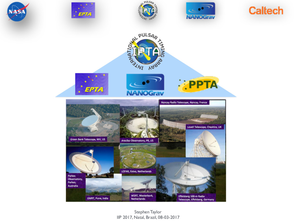
Searching for gravitational waves Supermassive black-hole binaries as sources of nanohertz gravitational waves Impact of binary environments on GW signals.
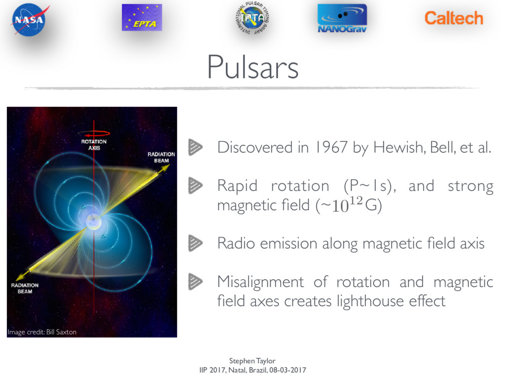
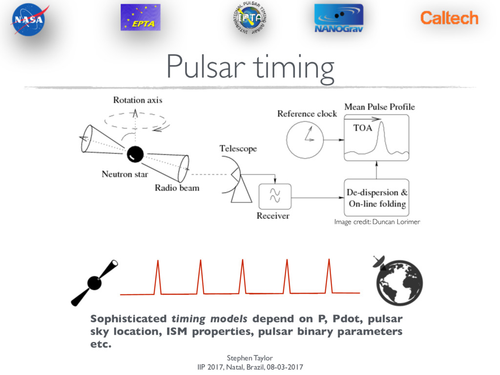
by Hewish, Bell, et al. Rapid rotation (P~1s), and strong magnetic field (~ G) Radio emission along magnetic field axis Misalignment of rotation and magnetic field axes creates lighthouse effect 1012 Image credit: Bill Saxton Pulsars
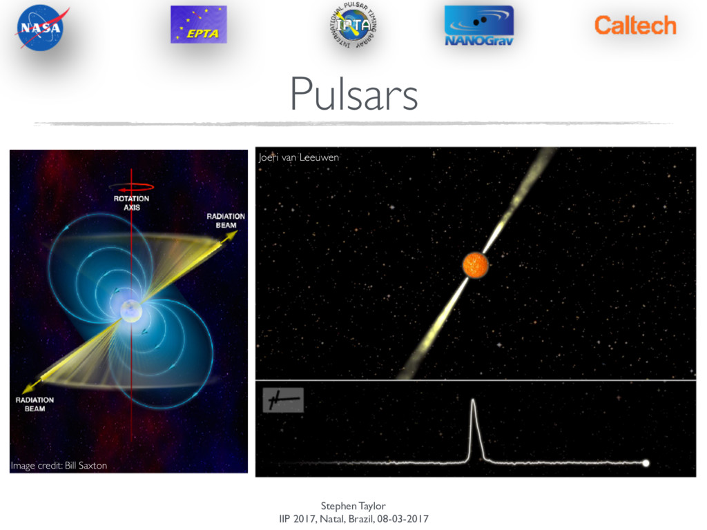
by Hewish, Bell, et al. Rapid rotation (P~1s), and strong magnetic field (~ G) Radio emission along magnetic field axis Misalignment of rotation and magnetic field axes creates lighthouse effect 1012 Image credit: Bill Saxton Joeri van Leeuwen Pulsars
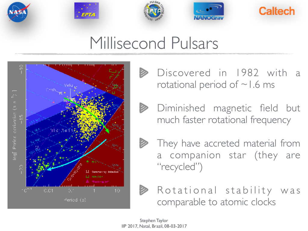
in 1982 with a rotational period of ~1.6 ms Diminished magnetic field but much faster rotational frequency They have accreted material from a companion star (they are “recycled”) R o t a t i o n a l s t a b i l i t y w a s comparable to atomic clocks
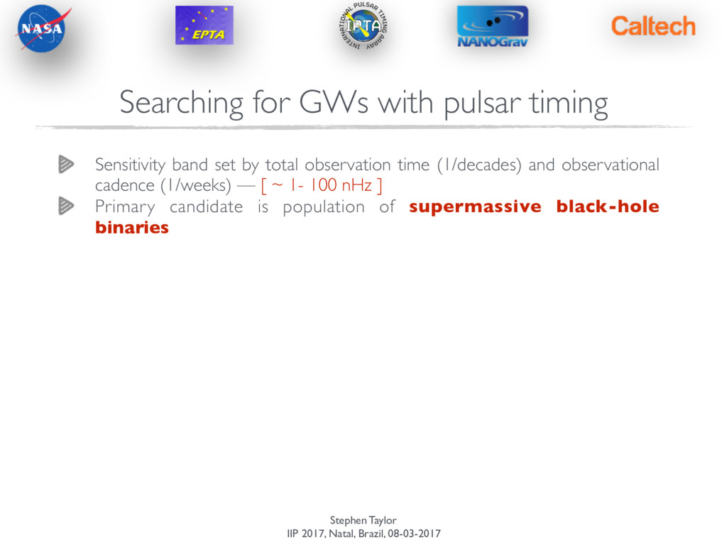
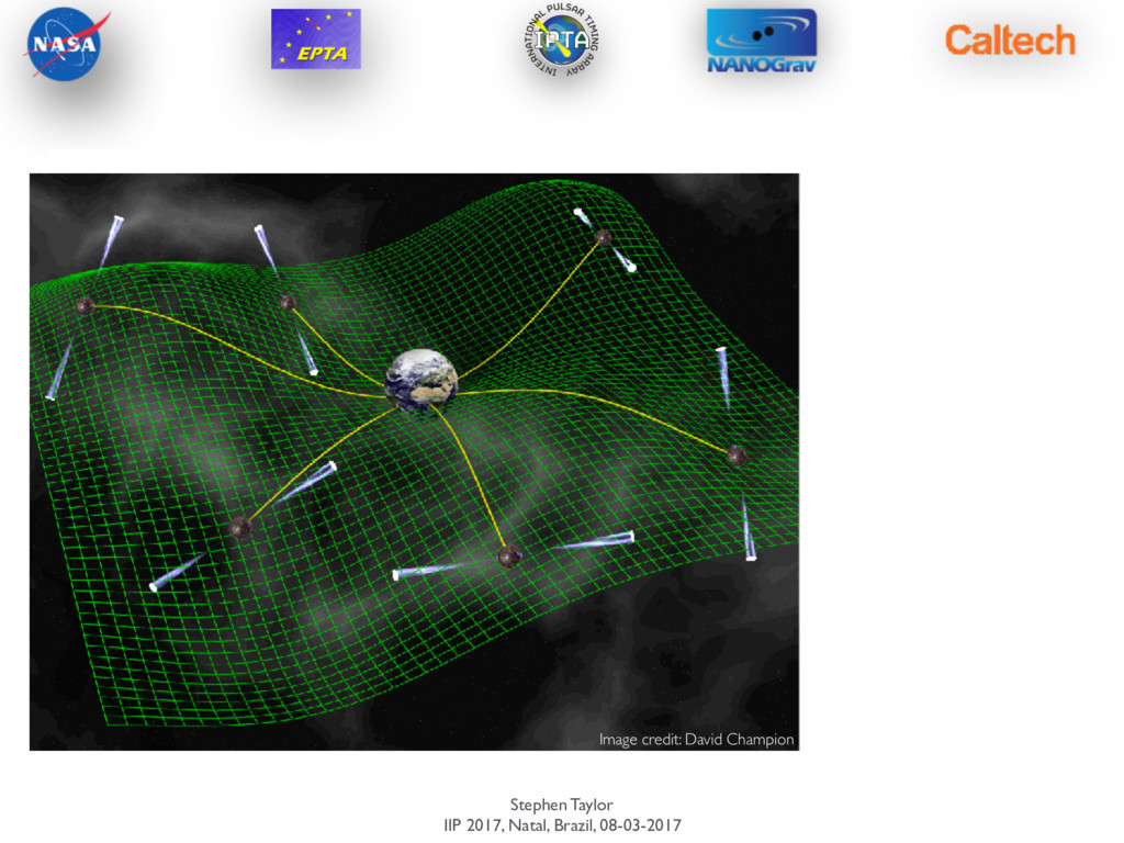
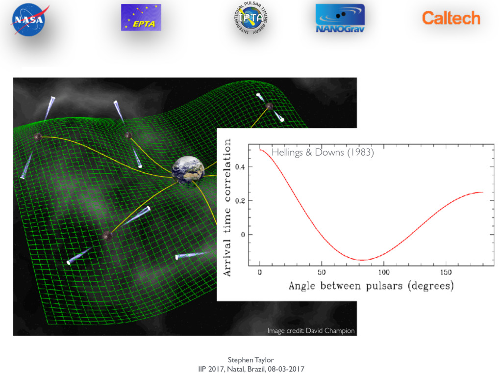
by total observation time (1/decades) and observational cadence (1/weeks) — [ ~ 1- 100 nHz ] Primary candidate is population of supermassive black-hole binaries Searching for GWs with pulsar timing
by total observation time (1/decades) and observational cadence (1/weeks) — [ ~ 1- 100 nHz ] Primary candidate is population of supermassive black-hole binaries Image credit: CSIRO Searching for GWs with pulsar timing
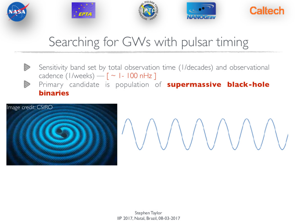
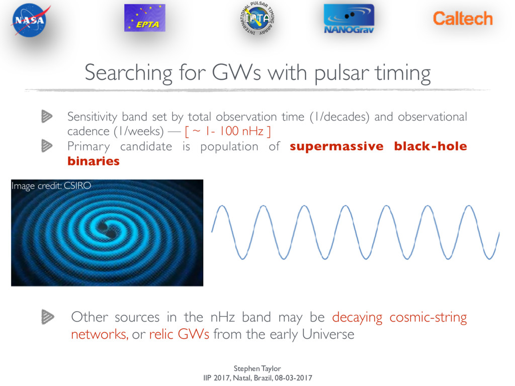
by total observation time (1/decades) and observational cadence (1/weeks) — [ ~ 1- 100 nHz ] Primary candidate is population of supermassive black-hole binaries Image credit: CSIRO Searching for GWs with pulsar timing
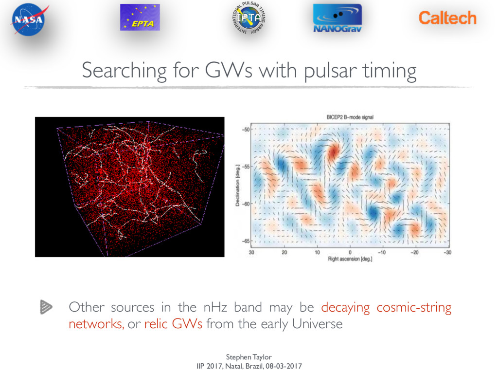
by total observation time (1/decades) and observational cadence (1/weeks) — [ ~ 1- 100 nHz ] Primary candidate is population of supermassive black-hole binaries Image credit: CSIRO Searching for GWs with pulsar timing Other sources in the nHz band may be decaying cosmic-string networks, or relic GWs from the early Universe
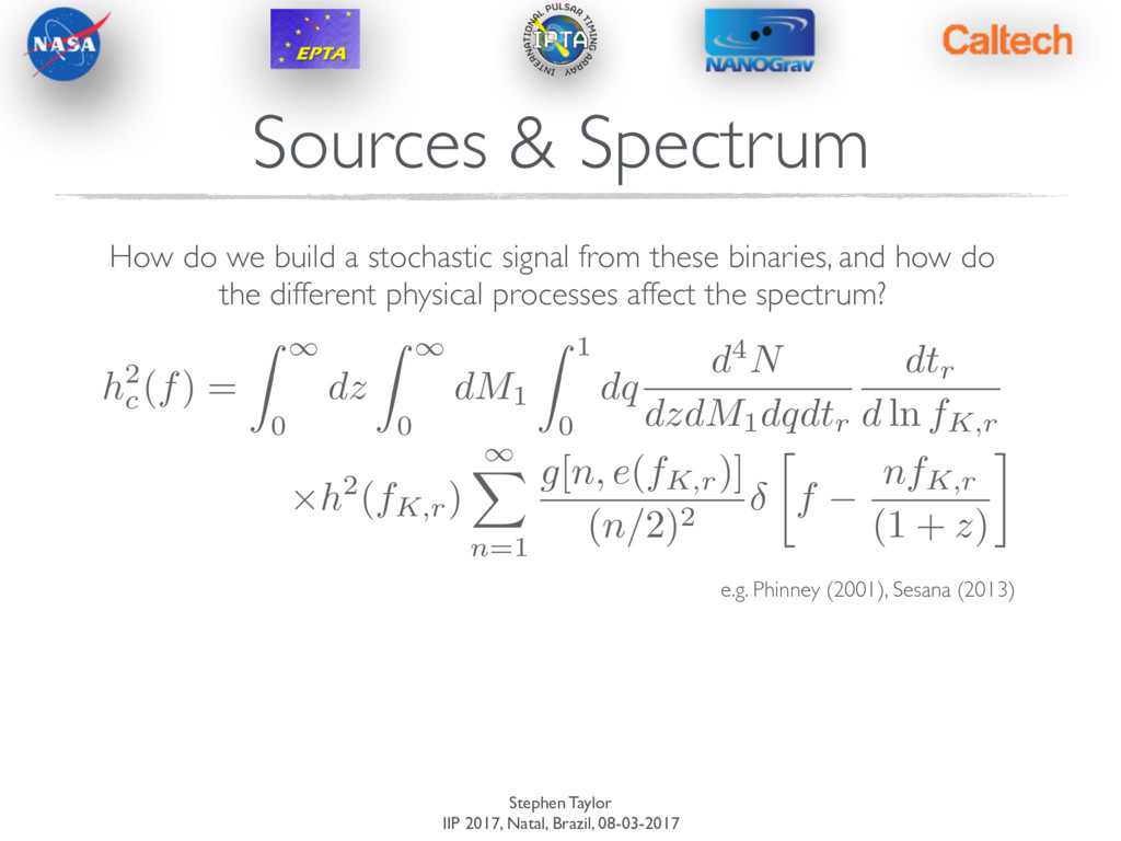
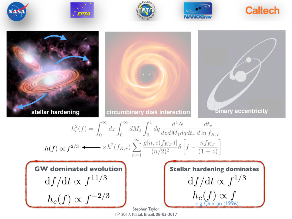
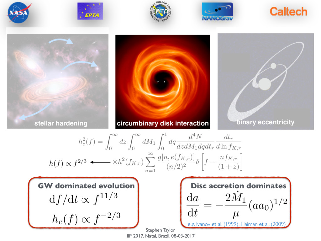
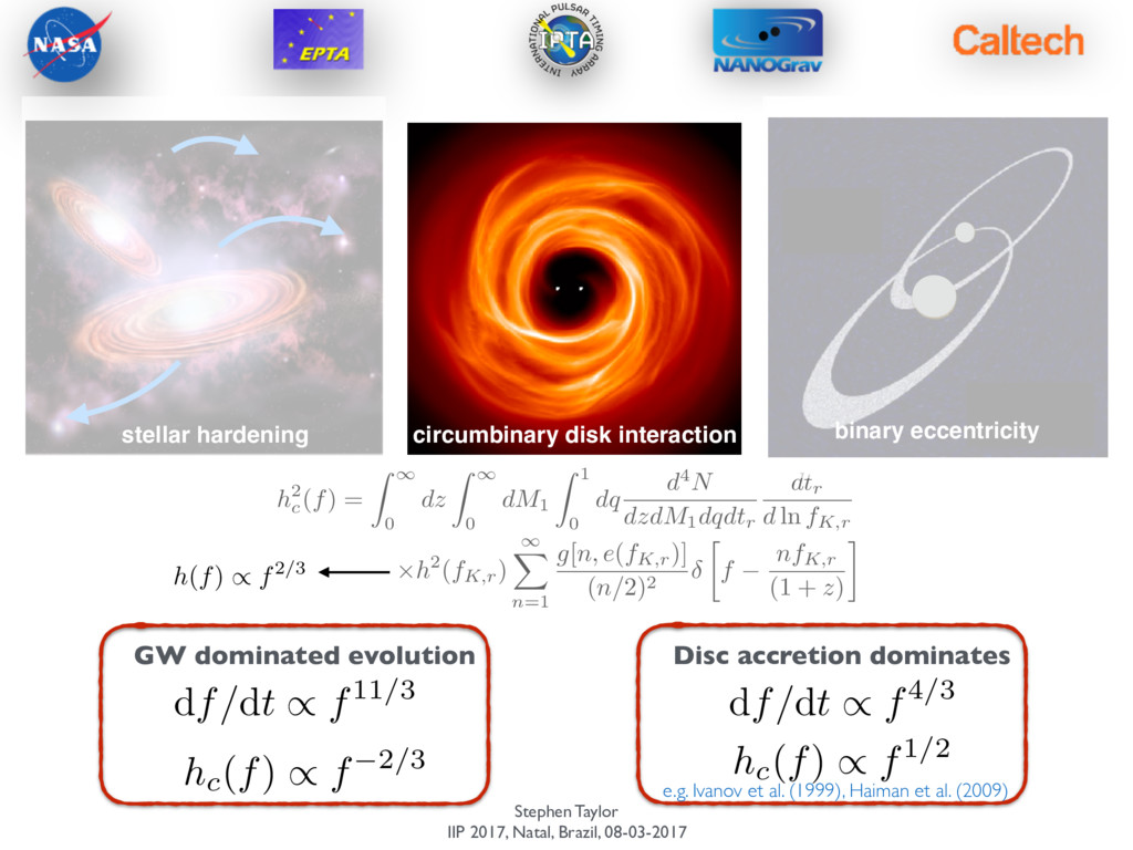
How do we build a stochastic signal from these binaries, and how do the different physical processes affect the spectrum? h2 c (f) = Z 1 0 dz Z 1 0 dM1 Z 1 0 dq d4N dzdM1dqdtr dtr d ln fK,r ⇥h2(fK,r) 1 X n=1 g[n, e(fK,r)] (n/2)2 f nfK,r (1 + z) e.g. Phinney (2001), Sesana (2013)
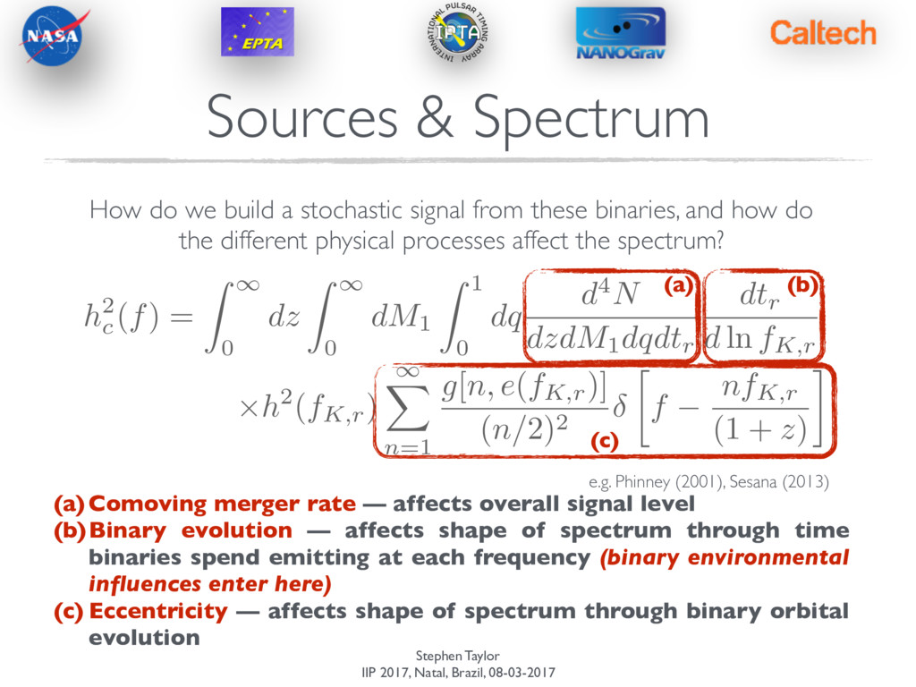
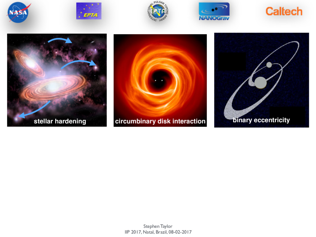
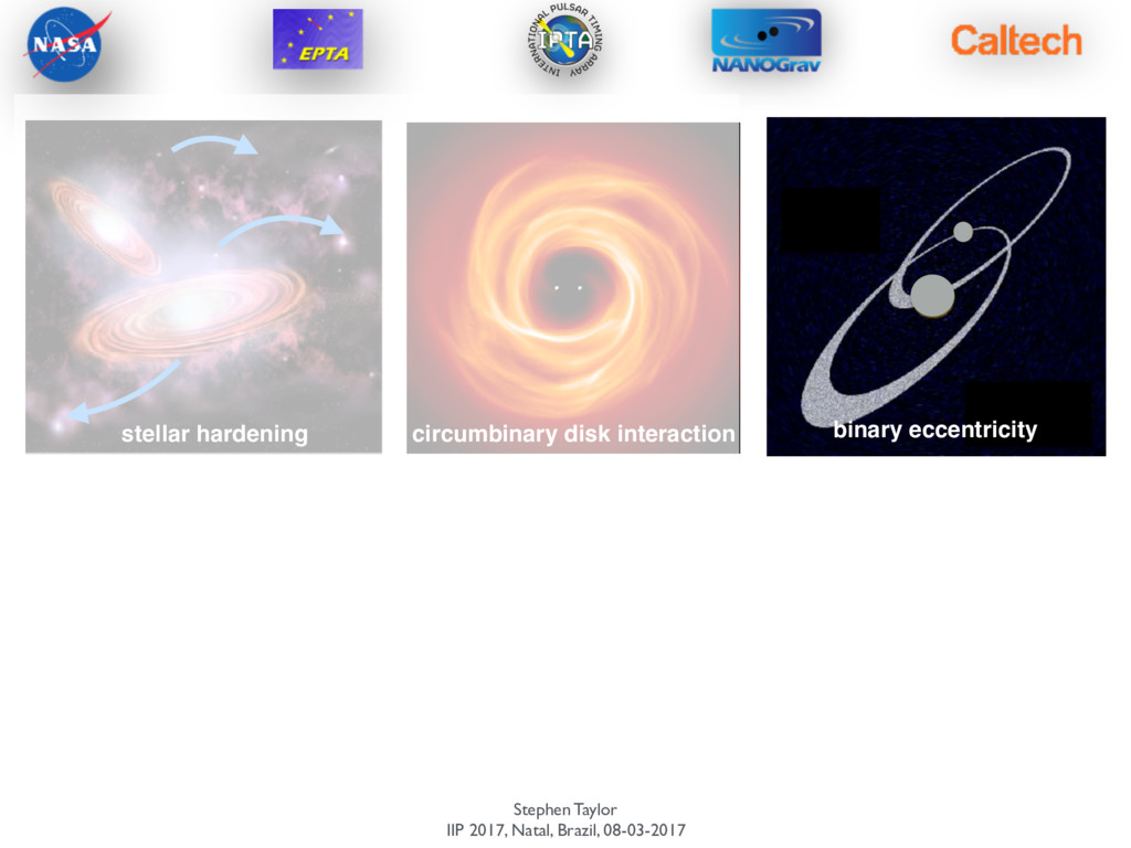
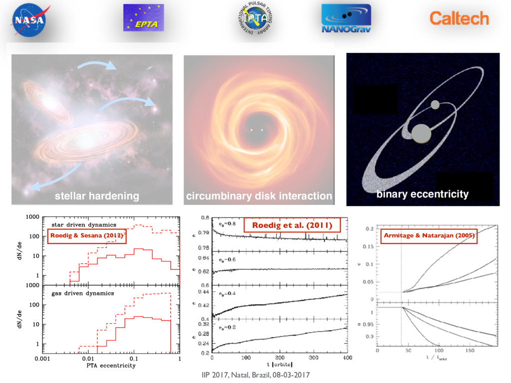
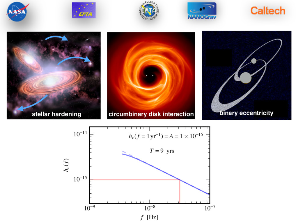
How do we build a stochastic signal from these binaries, and how do the different physical processes affect the spectrum? h2 c (f) = Z 1 0 dz Z 1 0 dM1 Z 1 0 dq d4N dzdM1dqdtr dtr d ln fK,r ⇥h2(fK,r) 1 X n=1 g[n, e(fK,r)] (n/2)2 f nfK,r (1 + z) e.g. Phinney (2001), Sesana (2013) (a) (b) (c) (a) Comoving merger rate — affects overall signal level (b)Binary evolution — affects shape of spectrum through time binaries spend emitting at each frequency (binary environmental influences enter here) (c) Eccentricity — affects shape of spectrum through binary orbital evolution
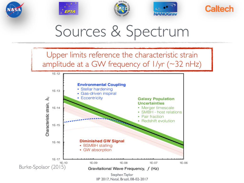
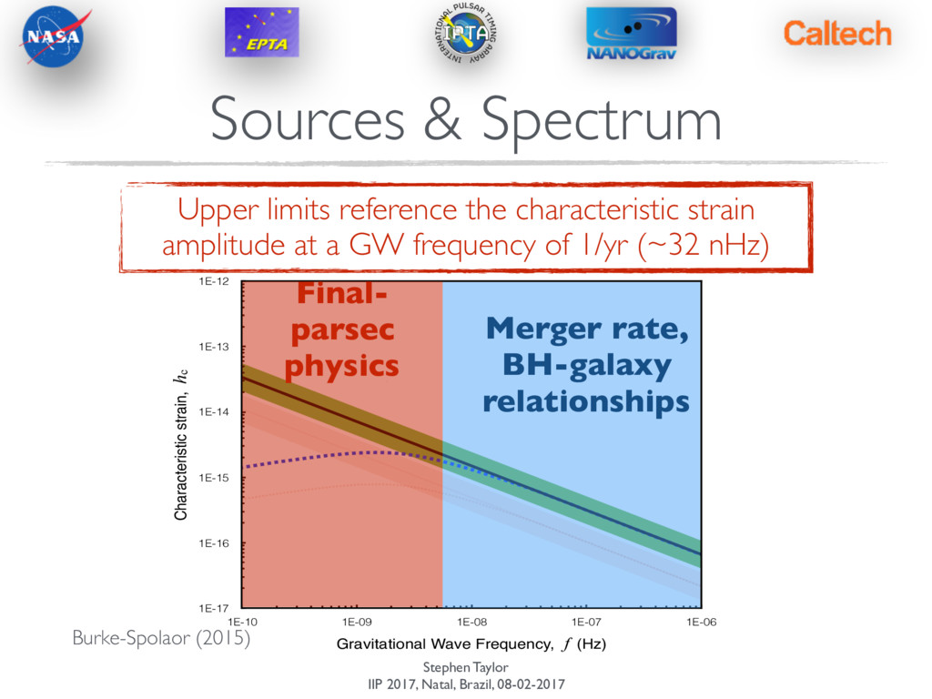
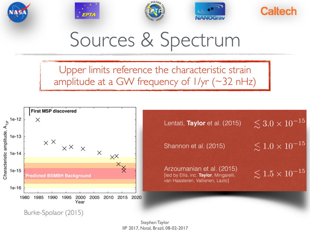
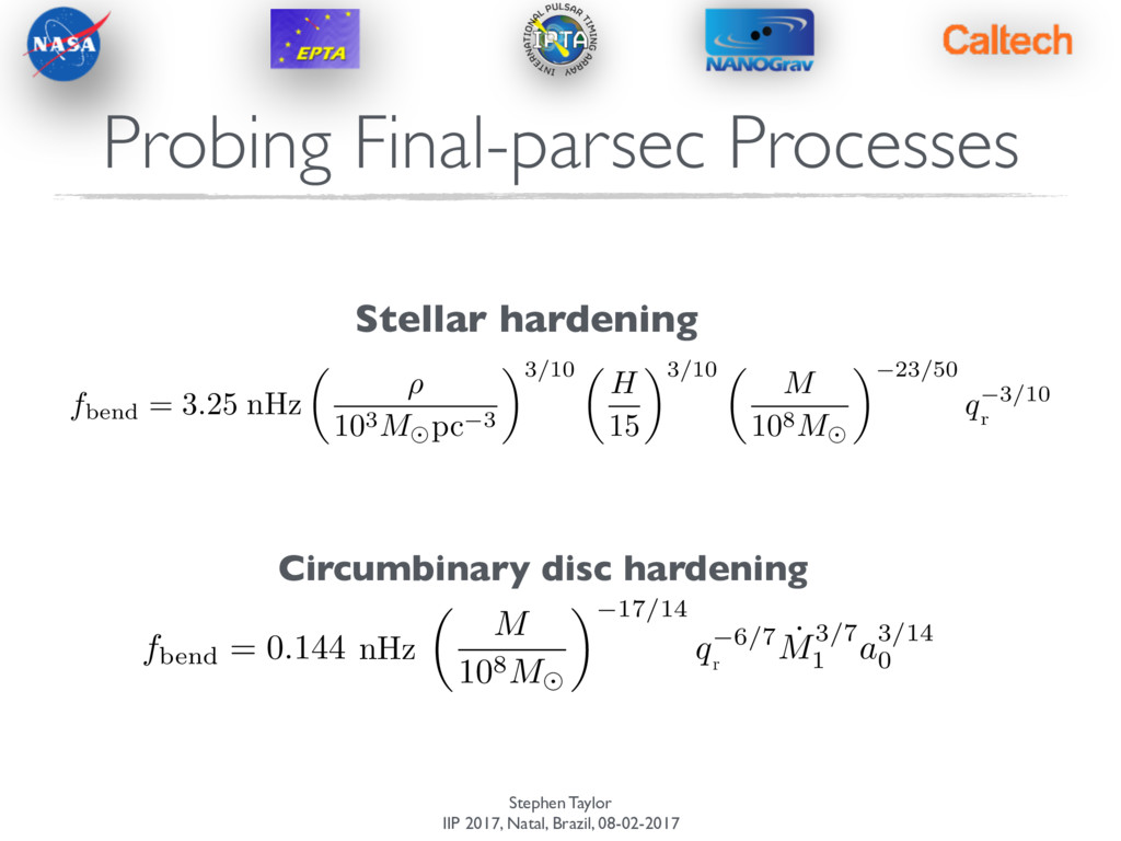
the characteristic strain amplitude at a GW frequency of 1/yr (~32 nHz) . 3.0 ⇥ 10 15 Environmental Coupling • Stellar hardening • Gas-driven inspiral • Eccentricity Galaxy Population Uncertainties • Merger timescale • SMBH - host relations • Pair fraction • Redshift evolution Diminished GW Signal • BSMBH stalling • GW absorption Characteristic strain, hc 1E-17 1E-16 1E-15 1E-14 1E-13 1E-12 Gravitational Wave Frequency, f (Hz) 1E-10 1E-09 1E-08 1E-07 1E-06 hc f 10.— A conceptual view of how various uncertainties in the BSMBH population and the GWs we can Burke-Spolaor (2015) Sources & Spectrum
the characteristic strain amplitude at a GW frequency of 1/yr (~32 nHz) . 3.0 ⇥ 10 15 Environmental Coupling • Stellar hardening • Gas-driven inspiral • Eccentricity Galaxy Population Uncertainties • Merger timescale • SMBH - host relations • Pair fraction • Redshift evolution Diminished GW Signal • BSMBH stalling • GW absorption Characteristic strain, hc 1E-17 1E-16 1E-15 1E-14 1E-13 1E-12 Gravitational Wave Frequency, f (Hz) 1E-10 1E-09 1E-08 1E-07 1E-06 hc f 10.— A conceptual view of how various uncertainties in the BSMBH population and the GWs we can Final- parsec physics Merger rate, BH-galaxy relationships Burke-Spolaor (2015) Sources & Spectrum
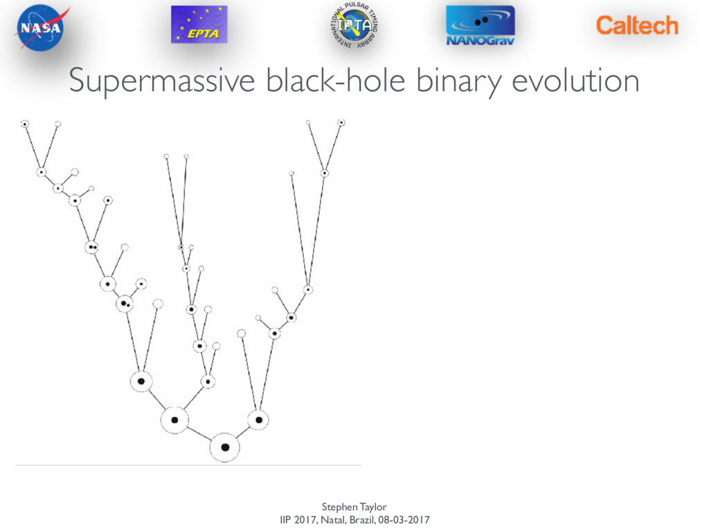
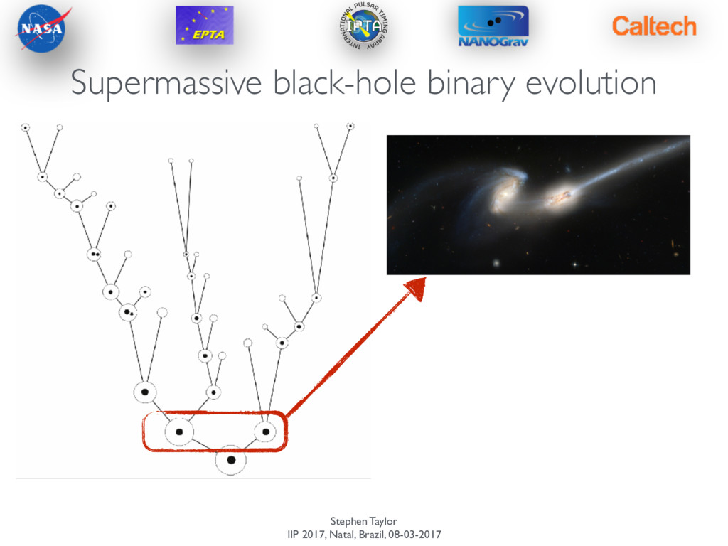
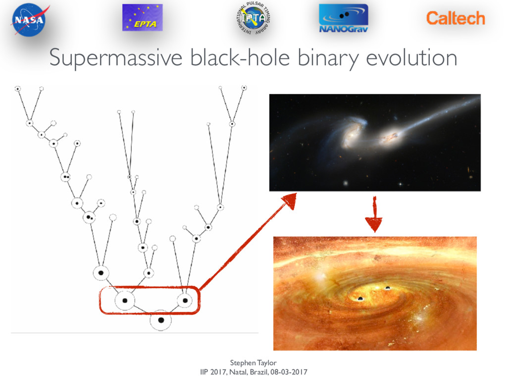
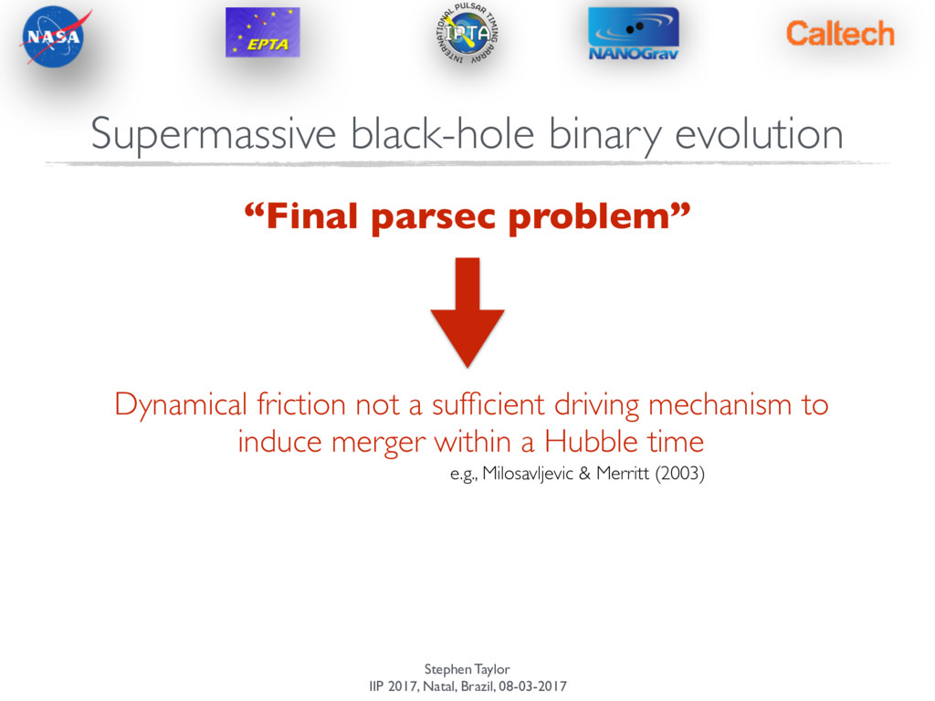
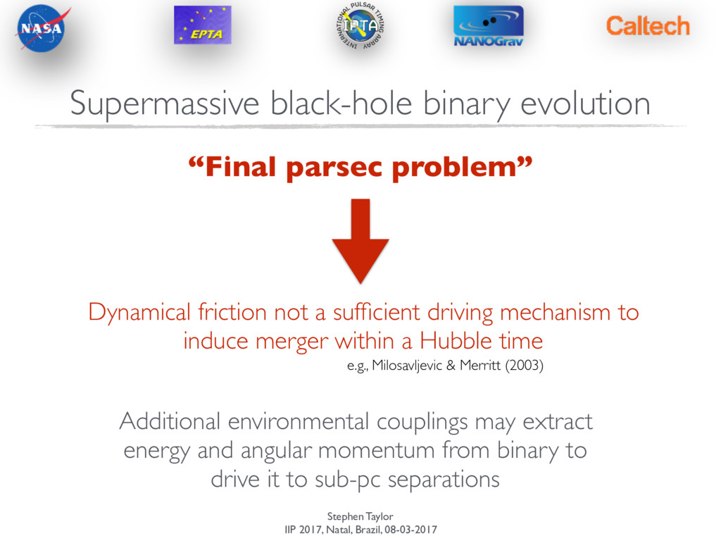
Dynamical friction not a sufficient driving mechanism to induce merger within a Hubble time e.g., Milosavljevic & Merritt (2003) Supermassive black-hole binary evolution
Dynamical friction not a sufficient driving mechanism to induce merger within a Hubble time e.g., Milosavljevic & Merritt (2003) Additional environmental couplings may extract energy and angular momentum from binary to drive it to sub-pc separations Supermassive black-hole binary evolution
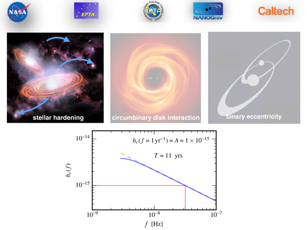
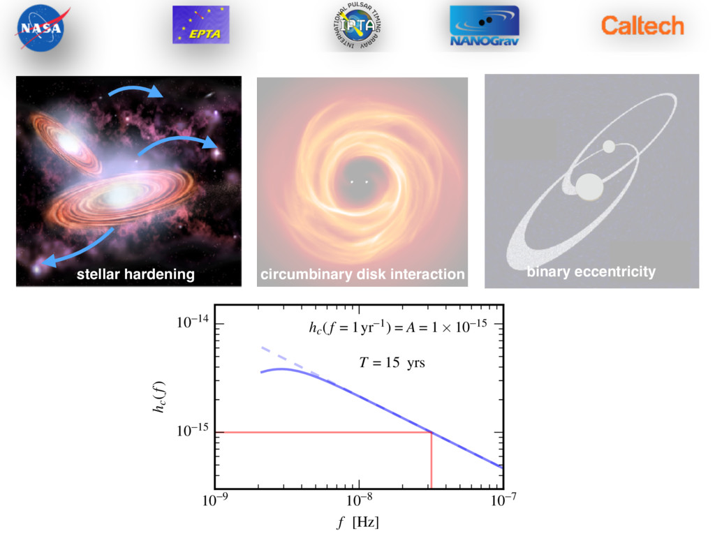
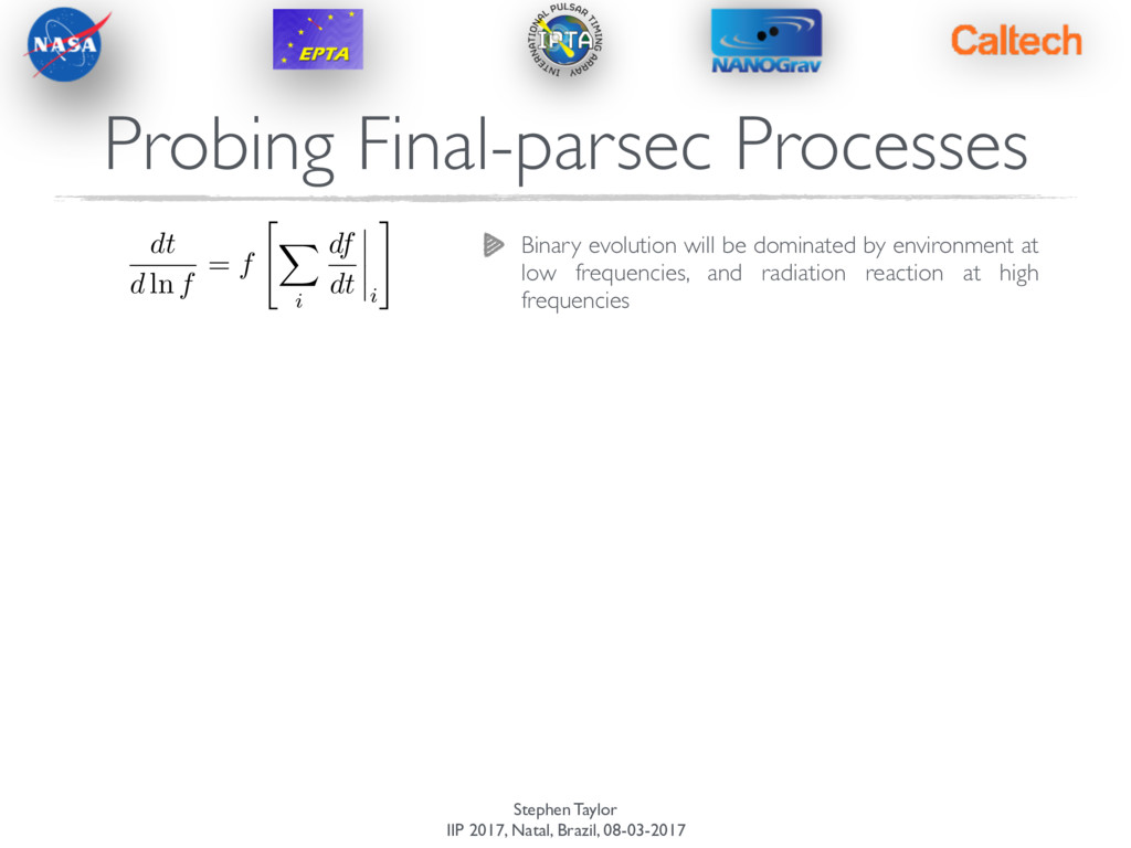
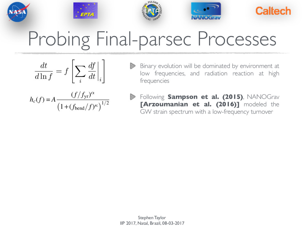
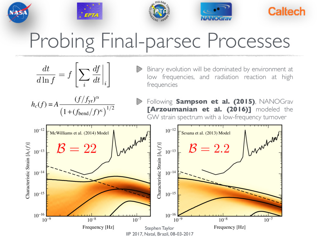
t/d ln f term) of this equation (see Colpi 2014, for a w of SMBHB coalescence). Following Sampson et al. 5) we can generalize the frequency dependence of the n spectrum to dt d ln f = f ✓ d f dt ◆-1 = f X i ✓ d f dt ◆ i !-1 , (23) e i ranges over many physical processes that are driv- he binary to coalescence. If we restrict this sum to GW- n evolution and an unspecified physical process then the n spectrum is now hc (f) = A (f/fyr )↵ 1+(fbend/f) 1/2 , (24) Binary evolution will be dominated by environment at low frequencies, and radiation reaction at high frequencies dt d ln f = f " X i df dt i # Following Sampson et al. (2015), NANOGrav [Arzoumanian et al. (2016)] modeled the GW strain spectrum with a low-frequency turnover
t/d ln f term) of this equation (see Colpi 2014, for a w of SMBHB coalescence). Following Sampson et al. 5) we can generalize the frequency dependence of the n spectrum to dt d ln f = f ✓ d f dt ◆-1 = f X i ✓ d f dt ◆ i !-1 , (23) e i ranges over many physical processes that are driv- he binary to coalescence. If we restrict this sum to GW- n evolution and an unspecified physical process then the n spectrum is now hc (f) = A (f/fyr )↵ 1+(fbend/f) 1/2 , (24) Binary evolution will be dominated by environment at low frequencies, and radiation reaction at high frequencies dt d ln f = f " X i df dt i # 12 10-9 10-8 10-7 Frequency [Hz] 10-16 10-15 10-14 10-13 10-12 Characteristic Strain [hc( f)] McWilliams et al. (2014) Model 10-9 10-8 10-7 Frequency [Hz] 10-16 10-15 10-14 10-13 10-12 Characteristic Strain [hc( f)] Sesana et al. (2013) Model Following Sampson et al. (2015), NANOGrav [Arzoumanian et al. (2016)] modeled the GW strain spectrum with a low-frequency turnover B = 22 B = 2.2
“Constraints On The Dynamical Environments Of Supermassive Black-hole Binaries Using Pulsar-timing Arrays”, Taylor, Simon, Sampson, arXiv:1612.02817, PRL 118, 181102 (2017) This approach can be adapted for LIGO and LISA population inference, to map from distributions of source properties back to progenitor characteristics. (Barrett et al., arXiv:1704.03781)
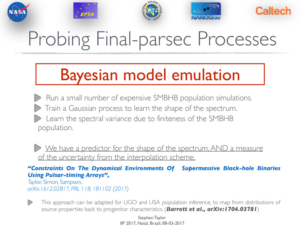
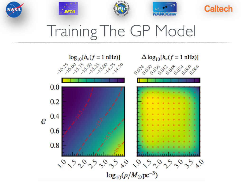
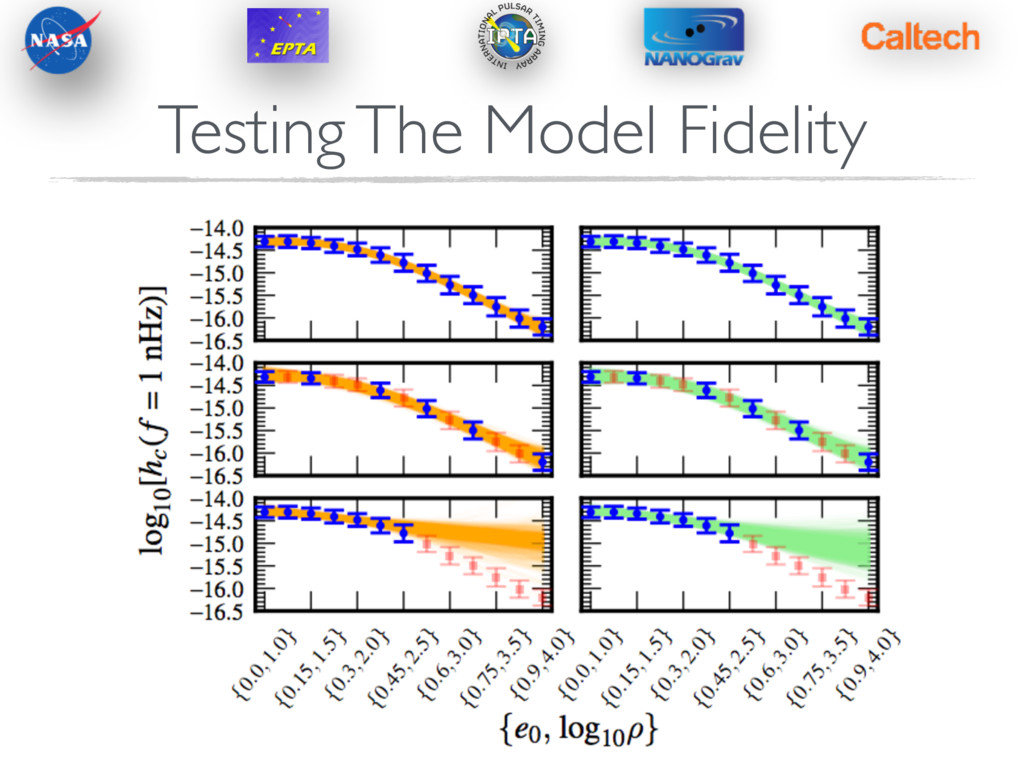
Run a small number of expensive SMBHB population simulations. Train a Gaussian process to learn the shape of the spectrum. Learn the spectral variance due to finiteness of the SMBHB population. We have a predictor for the shape of the spectrum, AND a measure of the uncertainty from the interpolation scheme. Probing Final-parsec Processes “Constraints On The Dynamical Environments Of Supermassive Black-hole Binaries Using Pulsar-timing Arrays”, Taylor, Simon, Sampson, arXiv:1612.02817, PRL 118, 181102 (2017) This approach can be adapted for LIGO and LISA population inference, to map from distributions of source properties back to progenitor characteristics. (Barrett et al., arXiv:1704.03781)
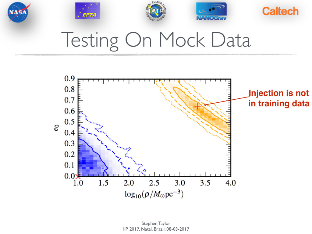
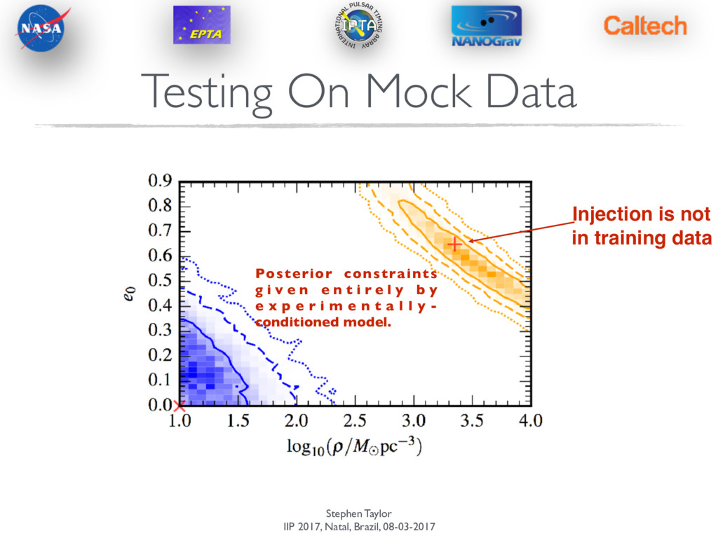
Data Posterior constraints given entirely by experimentally- conditioned model. Injection is not in training data Posterior constraints g i v e n e n t i r e l y b y e x p e r i m e n t a l l y - conditioned model.
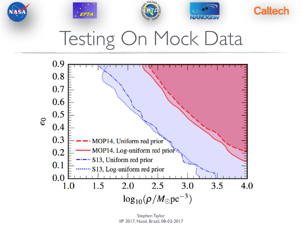
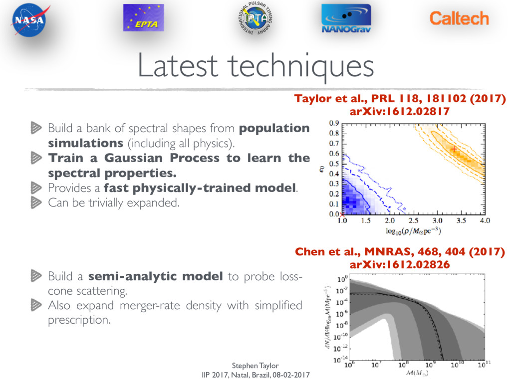
a bank of spectral shapes from population simulations (including all physics). Train a Gaussian Process to learn the spectral properties. Provides a fast physically-trained model. Can be trivially expanded. Build a semi-analytic model to probe loss- cone scattering. Also expand merger-rate density with simplified prescription. Taylor et al., PRL 118, 181102 (2017) arXiv:1612.02817 Chen et al., MNRAS, 468, 404 (2017) arXiv:1612.02826
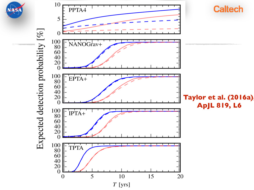
expected to make a GW detection within ~5-10 years. The GW strain spectrum encodes information about SMBHB dynamical evolution. Constraining the spectral shape can tell us about disc accretion, and loss-scone scattering. Gaussian Process emulation or semi-analytic methods allow direct reconstruction of SMBHB astrophysical environmental conditions.