Update On NANOGrav Data Analysis Techniques

Working group update given at International Pulsar Timing Array 2017 meeting in Sevres, France.

Transcript

1. UPDATE ON NANOGRAV DATA ANALYSIS TECHNIQUES Stephen Taylor JET PROPULSION LABORATORY, CALIFORNIA INSTITUTE OF TECHNOLOGY © 2017 California Institute of Technology. Government sponsorship acknowledged 1
2. 2 Overview publications since IPTA 2016 15 strong overlap of membership with LIGO & LISA communities
3. 3 1 2 3 4 NANOGrav 11yr dataset goals of the 11yr analysis analysis infrastructure preliminary results Overview
4. 4 NANOGRAV 11-YR DATASET
5. 5 pulsars NANOGrav 11yr Dataset 45 309,647 TOAs 11.4 years of observations (34 have timespans > 3 yrs) (27,571 from J1713+0747 alone)
6. 6 NANOGrav 11yr Dataset size ! NTOA color ! T obs
7. 7 GOALS OF THE 11-YR ANALYSIS
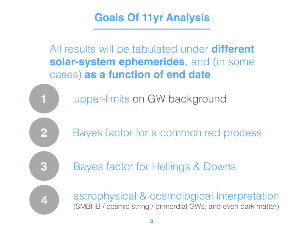
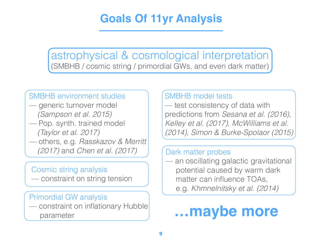
8. 8 1 2 upper-limits on GW background Bayes factor for a common red process Goals Of 11yr Analysis All results will be tabulated under different solar-system ephemerides, and (in some cases) as a function of end date 3 Bayes factor for Hellings & Downs 4 astrophysical & cosmological interpretation (SMBHB / cosmic string / primordial GWs, and even dark matter)
9. 9 Goals Of 11yr Analysis astrophysical & cosmological interpretation (SMBHB / cosmic string / primordial GWs, and even dark matter) SMBHB environment studies — generic turnover model (Sampson et al. 2015) — Pop. synth. trained model (Taylor et al. 2017) — others, e.g. Rasskazov & Merritt (2017) and Chen et al. (2017) SMBHB model tests — test consistency of data with predictions from Sesana et al. (2016), Kelley et al. (2017), McWilliams et al. (2014), Simon & Burke-Spolaor (2015) Cosmic string analysis — constraint on string tension Primordial GW analysis — constraint on inflationary Hubble parameter Dark matter probes — an oscillating galactic gravitational potential caused by warm dark matter can influence TOAs, e.g. Khmnelnitsky et al. (2014) …maybe more
10. 10 ANALYSIS INFRASTRUCTURE
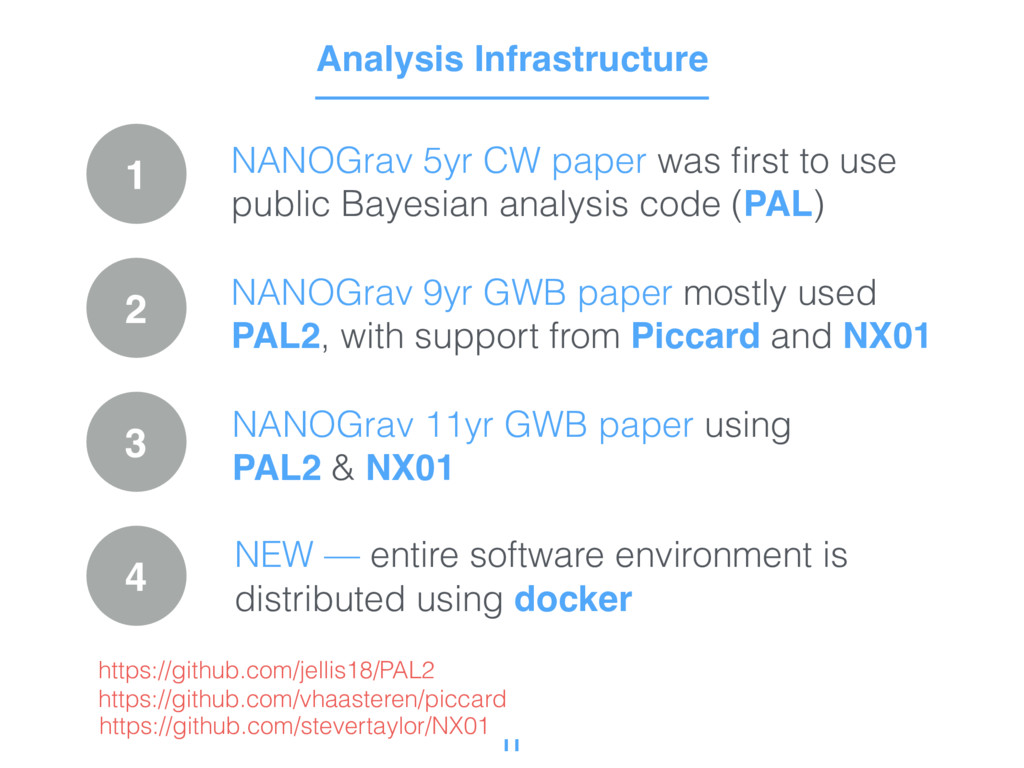
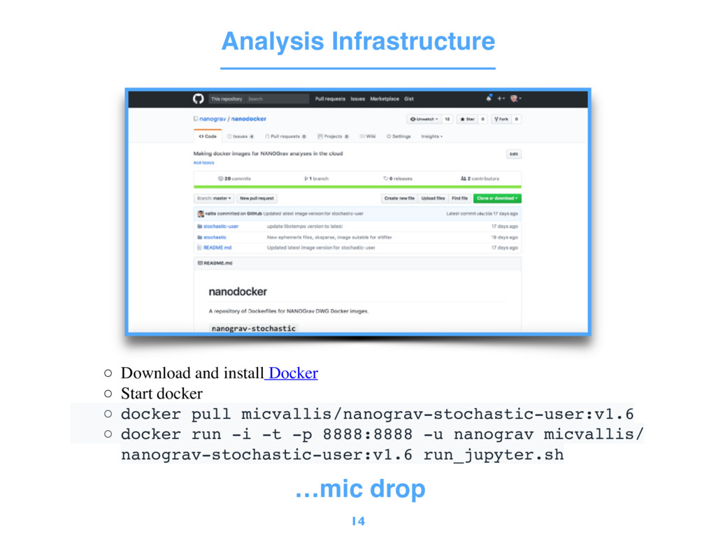
11. 11 1 2 3 NANOGrav 5yr CW paper was first to use public Bayesian analysis code (PAL) NANOGrav 9yr GWB paper mostly used PAL2, with support from Piccard and NX01 NANOGrav 11yr GWB paper using PAL2 & NX01 Analysis Infrastructure 4 NEW — entire software environment is distributed using docker https://github.com/stevertaylor/NX01 https://github.com/jellis18/PAL2 https://github.com/vhaasteren/piccard
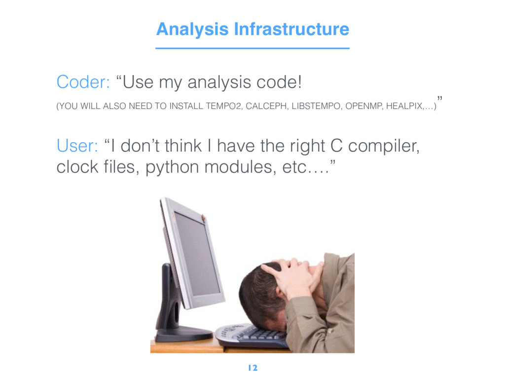
12. 12 Analysis Infrastructure Coder: “Use my analysis code! (YOU WILL ALSO NEED TO INSTALL TEMPO2, CALCEPH, LIBSTEMPO, OPENMP, HEALPIX,…) ” User: “I don’t think I have the right C compiler, clock files, python modules, etc….”
13. 13 Analysis Infrastructure Coder: “OK, use this docker image!” User: “…”
14. 14 Analysis Infrastructure ◦ Download and install Docker ◦ Start docker ◦ docker pull micvallis/nanograv-stochastic-user:v1.6 ◦ docker run -i -t -p 8888:8888 -u nanograv micvallis/ nanograv-stochastic-user:v1.6 run_jupyter.sh …mic drop
15. 15 PRELIMINARY RESULTS
16. 16 Members Of The DWG …and many more, including extensive collaboration with other working groups.
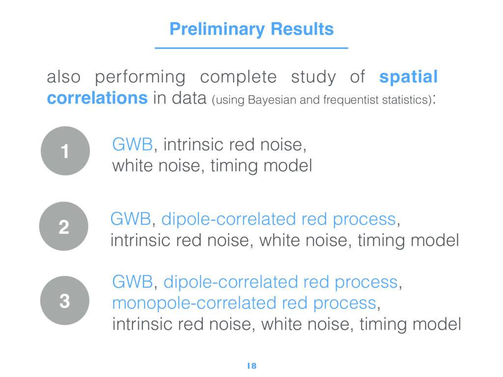
17. 10-9 10-8 10-7 Observed GW Frequency, f [Hz] 10-16 10-15 10-14 10-13 10-12 Characteristic Strain, hc( f ) Pessimistic [e.g. Sesana et al. (2016)] 17 upper limits and detection statistics are sensitive to our choice of ephemeris model Preliminary Results results produced by ~5-10 people with the nanodocker image blue = common red process, orange = H&D red process
18. 18 also performing complete study of spatial correlations in data (using Bayesian and frequentist statistics): Preliminary Results 1 2 3 GWB, intrinsic red noise, white noise, timing model GWB, dipole-correlated red process, intrinsic red noise, white noise, timing model GWB, dipole-correlated red process, monopole-correlated red process, intrinsic red noise, white noise, timing model
19. 19 BONUS
20. 20 Introducing Enterprise Enhanced Numerical Toolbox Enabling a Robust PulsaR Inference SuitE see Paul Baker’s talk today @ 3.40pm https://enterprise.readthedocs.io
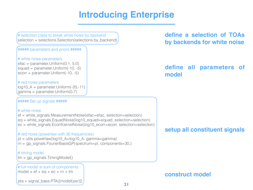
21. 21 Introducing Enterprise # selection class to break white noise by backend selection = selections.Selection(selections.by_backend) ##### parameters and priors ##### # white noise parameters efac = parameter.Uniform(0.1, 5.0) equad = parameter.Uniform(-10, -5) ecorr = parameter.Uniform(-10, -5) # red noise parameters log10_A = parameter.Uniform(-20,-11) gamma = parameter.Uniform(0,7) ##### Set up signals ##### # white noise ef = white_signals.MeasurementNoise(efac=efac, selection=selection) eq = white_signals.EquadNoise(log10_equad=equad, selection=selection) ec = white_signals.EcorrKernelNoise(log10_ecorr=ecorr, selection=selection) # red noise (powerlaw with 30 frequencies) pl = utils.powerlaw(log10_A=log10_A, gamma=gamma) rn = gp_signals.FourierBasisGP(spectrum=pl, components=30,) # timing model tm = gp_signals.TimingModel() # full model is sum of components model = ef + eq + ec + rn + tm pta = signal_base.PTA([model(psr)]) define a selection of TOAs by backends for white noise define all parameters of model setup all constituent signals construct model