Institute of Technology. Government sponsorship acknowledged Stephen Taylor Bayesian Inference for PTAs JET PROPULSION LABORATORY, CALIFORNIA INSTITUTE OF TECHNOLOGY
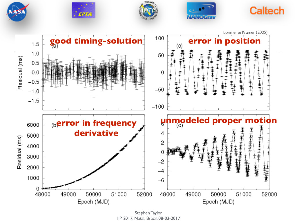
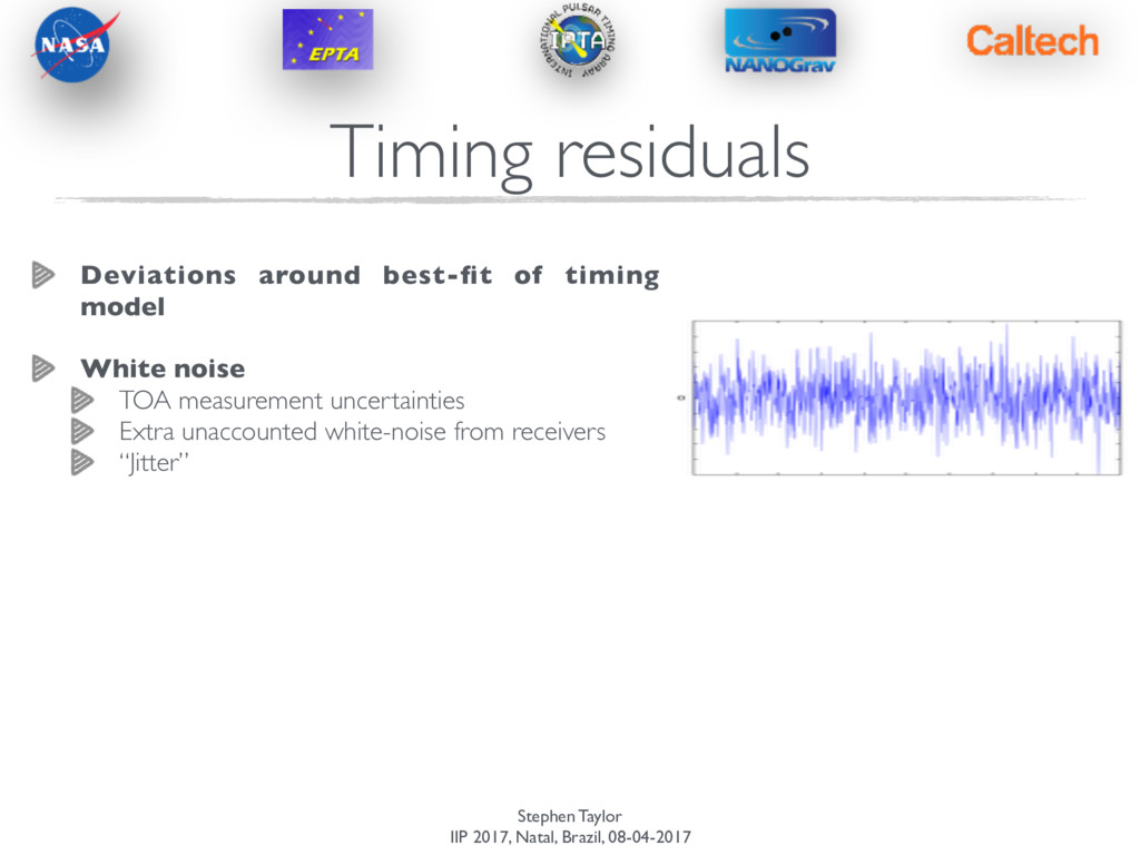
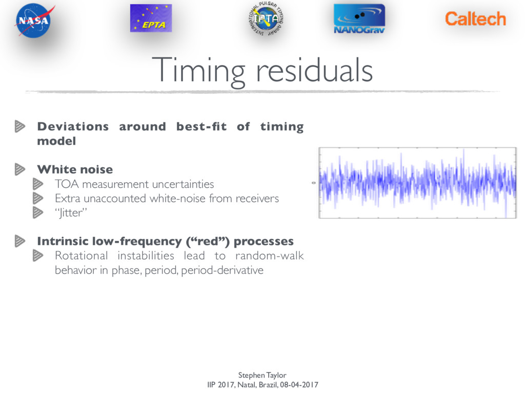
around best-fit of timing model White noise TOA measurement uncertainties Extra unaccounted white-noise from receivers “Jitter” Intrinsic low-frequency (“red”) processes Rotational instabilities lead to random-walk behavior in phase, period, period-derivative
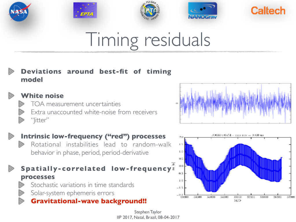
around best-fit of timing model White noise TOA measurement uncertainties Extra unaccounted white-noise from receivers “Jitter” Intrinsic low-frequency (“red”) processes Rotational instabilities lead to random-walk behavior in phase, period, period-derivative Spatially-correlated low-frequency processes Stochastic variations in time standards Solar-system ephemeris errors Gravitational-wave background!!
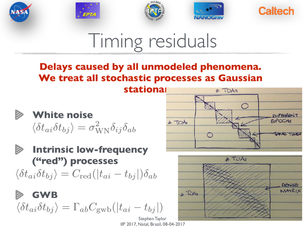
Delays caused by all unmodeled phenomena. We treat all stochastic processes as Gaussian stationary. White noise Intrinsic low-frequency (“red”) processes h tai tbj i = 2 WN ij ab h tai tbj i = Cred(|tai tbj |) ab h tai tbj i = abCgwb(|tai tbj |)
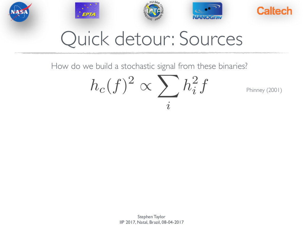
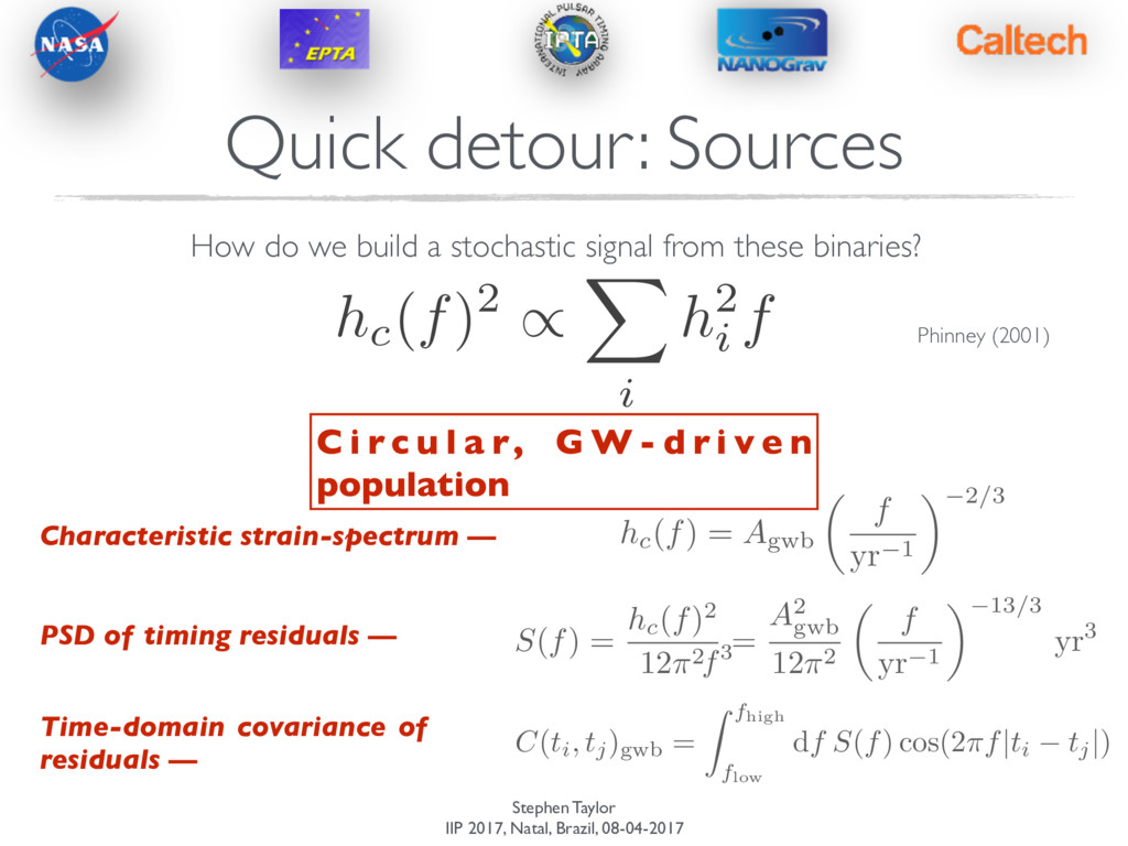
build a stochastic signal from these binaries? Phinney (2001) hc(f)2 / X i h2 i f C i r c u l a r, G W - d r i v e n population Quick detour: Sources Characteristic strain-spectrum — PSD of timing residuals — S(f) = hc(f)2 12⇡2 = A2 gwb 12⇡2 ✓ f yr 1 ◆ 13/3 yr3 hc(f) = Agwb ✓ f yr 1 ◆ 2/3 Time-domain covariance of residuals — C ( ti, tj)gwb = Z f high f low d f S ( f ) cos(2 ⇡f|ti tj | ) f3
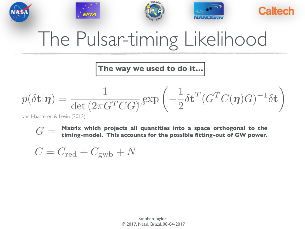
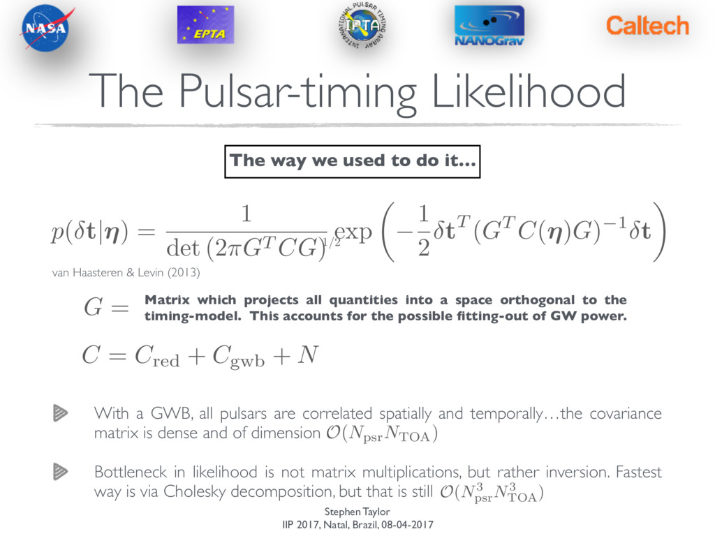
Levin (2013) The Pulsar-timing Likelihood p ( t|⌘ ) = 1 det (2 ⇡GT CG ) exp ✓ 1 2 tT ( GT C ( ⌘ ) G ) 1 t ◆ The way we used to do it… Matrix which projects all quantities into a space orthogonal to the timing-model. This accounts for the possible fitting-out of GW power. G = C = Cred + Cgwb + N 1/2
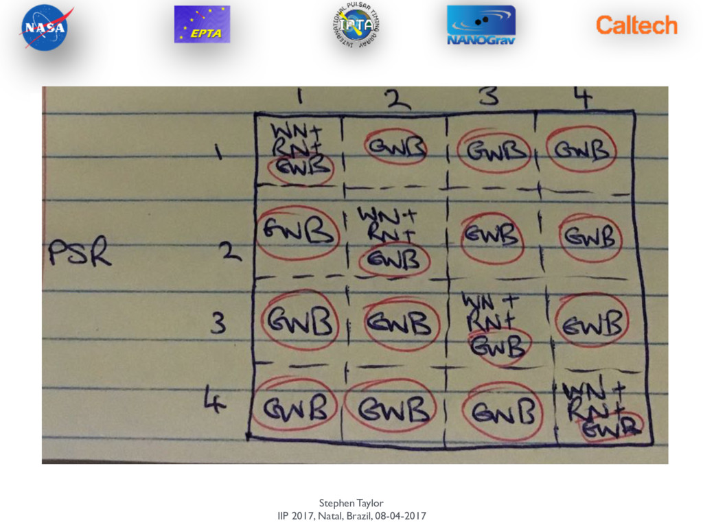
Levin (2013) The Pulsar-timing Likelihood p ( t|⌘ ) = 1 det (2 ⇡GT CG ) exp ✓ 1 2 tT ( GT C ( ⌘ ) G ) 1 t ◆ The way we used to do it… Matrix which projects all quantities into a space orthogonal to the timing-model. This accounts for the possible fitting-out of GW power. G = C = Cred + Cgwb + N 1/2 O(NpsrNTOA) With a GWB, all pulsars are correlated spatially and temporally…the covariance matrix is dense and of dimension Bottleneck in likelihood is not matrix multiplications, but rather inversion. Fastest way is via Cholesky decomposition, but that is still O(N3 psr N3 TOA )
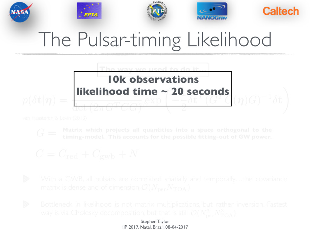
Levin (2013) The Pulsar-timing Likelihood p ( t|⌘ ) = 1 det (2 ⇡GT CG ) exp ✓ 1 2 tT ( GT C ( ⌘ ) G ) 1 t ◆ The way we used to do it… Matrix which projects all quantities into a space orthogonal to the timing-model. This accounts for the possible fitting-out of GW power. G = C = Cred + Cgwb + N 1/2 O(NpsrNTOA) With a GWB, all pulsars are correlated spatially and temporally…the covariance matrix is dense and of dimension Bottleneck in likelihood is not matrix multiplications, but rather inversion. Fastest way is via Cholesky decomposition, but that is still O(N3 psr N3 TOA ) 10k observations likelihood time ~ 20 seconds
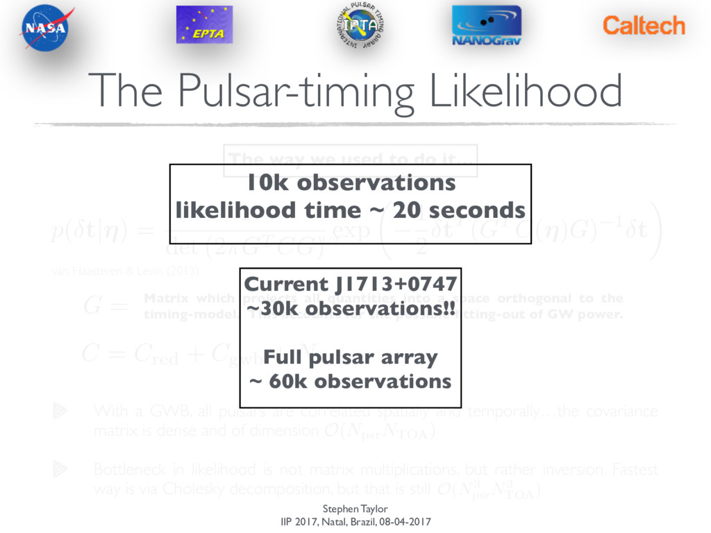
Levin (2013) The Pulsar-timing Likelihood p ( t|⌘ ) = 1 det (2 ⇡GT CG ) exp ✓ 1 2 tT ( GT C ( ⌘ ) G ) 1 t ◆ The way we used to do it… Matrix which projects all quantities into a space orthogonal to the timing-model. This accounts for the possible fitting-out of GW power. G = C = Cred + Cgwb + N 1/2 O(NpsrNTOA) With a GWB, all pulsars are correlated spatially and temporally…the covariance matrix is dense and of dimension Bottleneck in likelihood is not matrix multiplications, but rather inversion. Fastest way is via Cholesky decomposition, but that is still O(N3 psr N3 TOA ) 10k observations likelihood time ~ 20 seconds Current J1713+0747 ~30k observations!! Full pulsar array ~ 60k observations
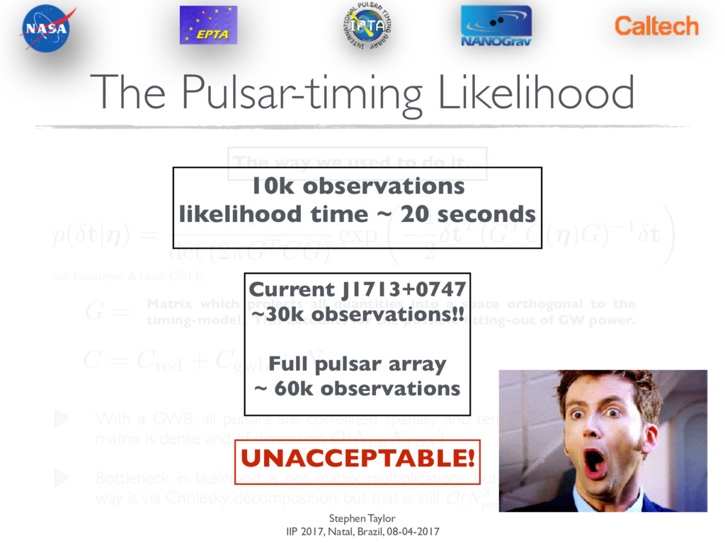
Levin (2013) The Pulsar-timing Likelihood p ( t|⌘ ) = 1 det (2 ⇡GT CG ) exp ✓ 1 2 tT ( GT C ( ⌘ ) G ) 1 t ◆ The way we used to do it… Matrix which projects all quantities into a space orthogonal to the timing-model. This accounts for the possible fitting-out of GW power. G = C = Cred + Cgwb + N 1/2 O(NpsrNTOA) With a GWB, all pulsars are correlated spatially and temporally…the covariance matrix is dense and of dimension Bottleneck in likelihood is not matrix multiplications, but rather inversion. Fastest way is via Cholesky decomposition, but that is still O(N3 psr N3 TOA ) 10k observations likelihood time ~ 20 seconds Current J1713+0747 ~30k observations!! Full pulsar array ~ 60k observations UNACCEPTABLE!
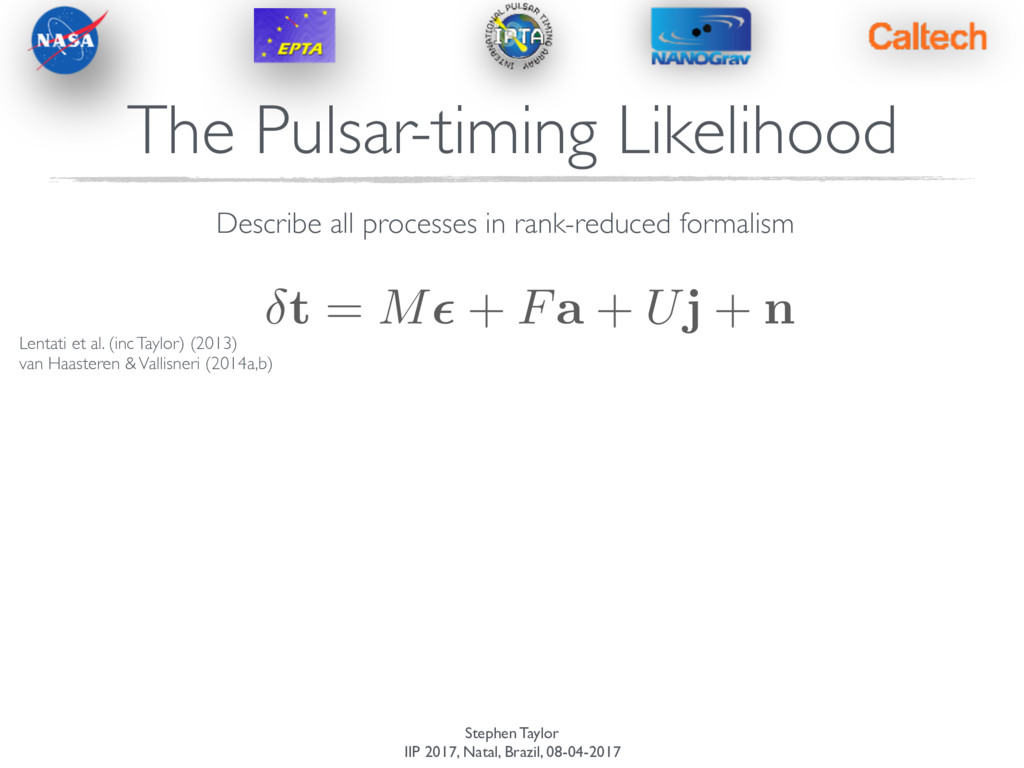
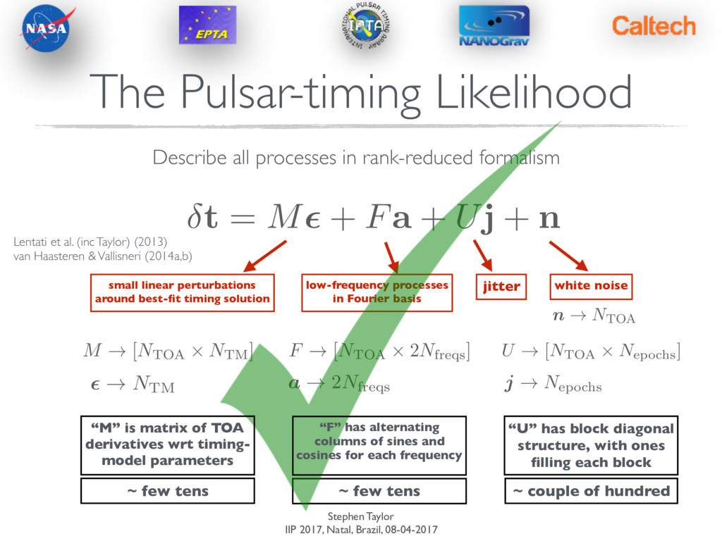
+ Fa + Uj + n The Pulsar-timing Likelihood Describe all processes in rank-reduced formalism Lentati et al. (inc Taylor) (2013) van Haasteren & Vallisneri (2014a,b)
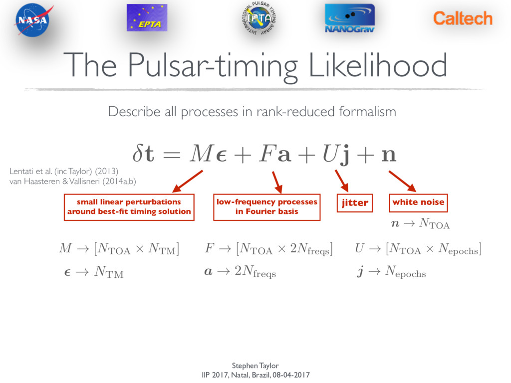
+ Fa + Uj + n The Pulsar-timing Likelihood Describe all processes in rank-reduced formalism small linear perturbations around best-fit timing solution low-frequency processes in Fourier basis jitter white noise Lentati et al. (inc Taylor) (2013) van Haasteren & Vallisneri (2014a,b)
+ Fa + Uj + n The Pulsar-timing Likelihood Describe all processes in rank-reduced formalism small linear perturbations around best-fit timing solution low-frequency processes in Fourier basis jitter white noise M ! [NTOA ⇥ NTM] ✏ ! NTM F ! [NTOA ⇥ 2Nfreqs] a ! 2Nfreqs U ! [NTOA ⇥ Nepochs] j ! N epochs n ! NTOA Lentati et al. (inc Taylor) (2013) van Haasteren & Vallisneri (2014a,b)
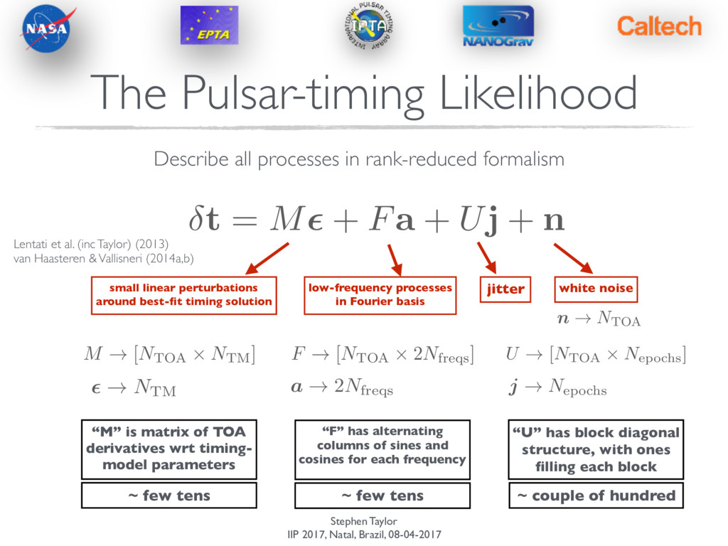
+ Fa + Uj + n The Pulsar-timing Likelihood Describe all processes in rank-reduced formalism small linear perturbations around best-fit timing solution low-frequency processes in Fourier basis jitter white noise M ! [NTOA ⇥ NTM] ✏ ! NTM F ! [NTOA ⇥ 2Nfreqs] a ! 2Nfreqs U ! [NTOA ⇥ Nepochs] j ! N epochs n ! NTOA ~ few tens ~ few tens ~ couple of hundred “M” is matrix of TOA derivatives wrt timing- model parameters “F” has alternating columns of sines and cosines for each frequency “U” has block diagonal structure, with ones filling each block Lentati et al. (inc Taylor) (2013) van Haasteren & Vallisneri (2014a,b)
+ Fa + Uj + n The Pulsar-timing Likelihood Describe all processes in rank-reduced formalism small linear perturbations around best-fit timing solution low-frequency processes in Fourier basis jitter white noise M ! [NTOA ⇥ NTM] ✏ ! NTM F ! [NTOA ⇥ 2Nfreqs] a ! 2Nfreqs U ! [NTOA ⇥ Nepochs] j ! N epochs n ! NTOA ~ few tens ~ few tens ~ couple of hundred “M” is matrix of TOA derivatives wrt timing- model parameters “F” has alternating columns of sines and cosines for each frequency “U” has block diagonal structure, with ones filling each block Lentati et al. (inc Taylor) (2013) van Haasteren & Vallisneri (2014a,b)
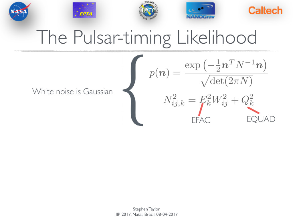
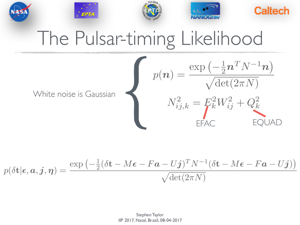
p ( n ) = exp 1 2 nT N 1n p det(2 ⇡N ) White noise is Gaussian N2 ij,k = E2 k W2 ij + Q2 k EFAC EQUAD p ( t|✏, a, j, ⌘ ) = exp 1 2 ( t M✏ Fa Uj ) T N 1 ( t M✏ Fa Uj ) p det(2 ⇡N )
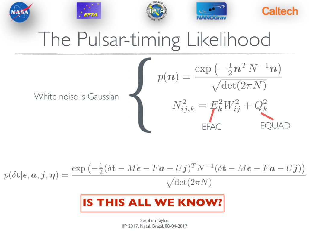
p ( n ) = exp 1 2 nT N 1n p det(2 ⇡N ) White noise is Gaussian N2 ij,k = E2 k W2 ij + Q2 k EFAC EQUAD p ( t|✏, a, j, ⌘ ) = exp 1 2 ( t M✏ Fa Uj ) T N 1 ( t M✏ Fa Uj ) p det(2 ⇡N ) IS THIS ALL WE KNOW?
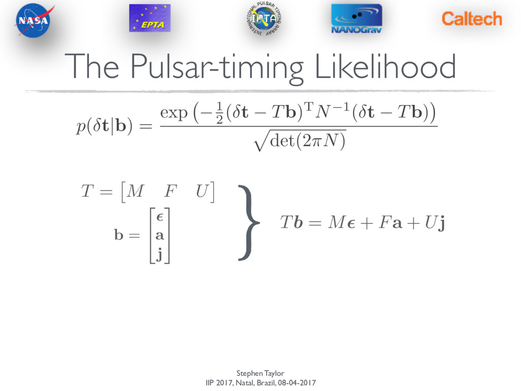
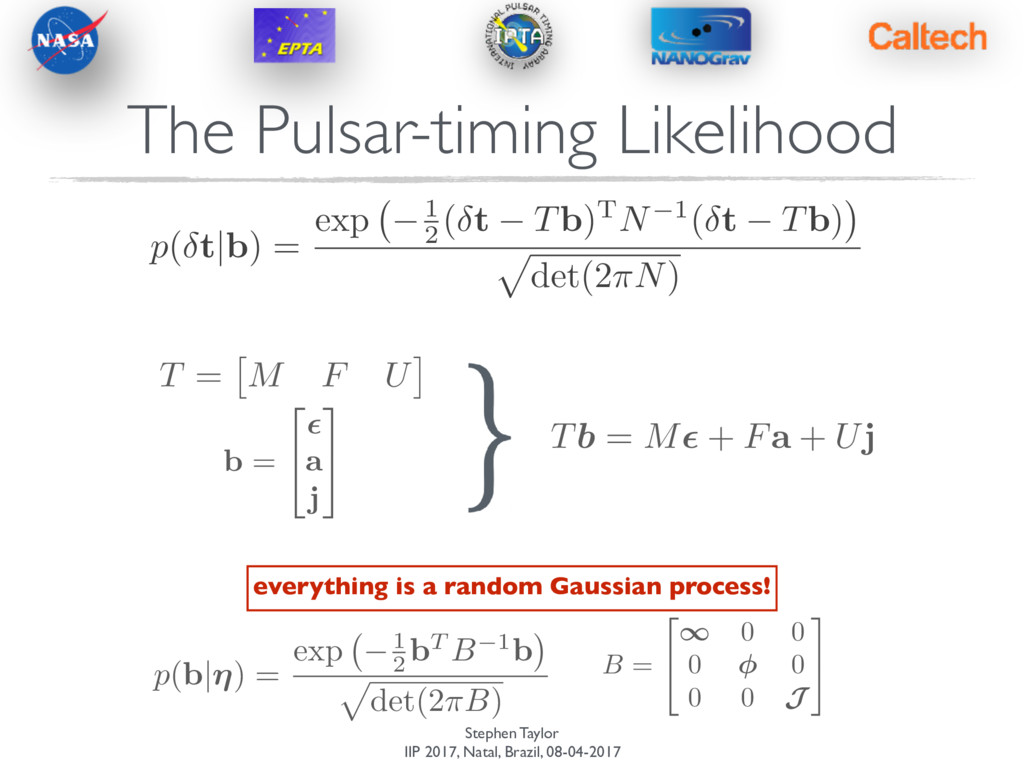
T = ⇥ M F U ⇤ b = 2 4 ✏ a j 3 5 Tb = M✏ + Fa + Uj p ( b|⌘ ) = exp 1 2 bT B 1b p det(2 ⇡B ) B = 2 4 1 0 0 0 0 0 0 J 3 5 p ( t|b ) = exp 1 2 ( t Tb ) TN 1 ( t Tb ) p det(2 ⇡N ) everything is a random Gaussian process!
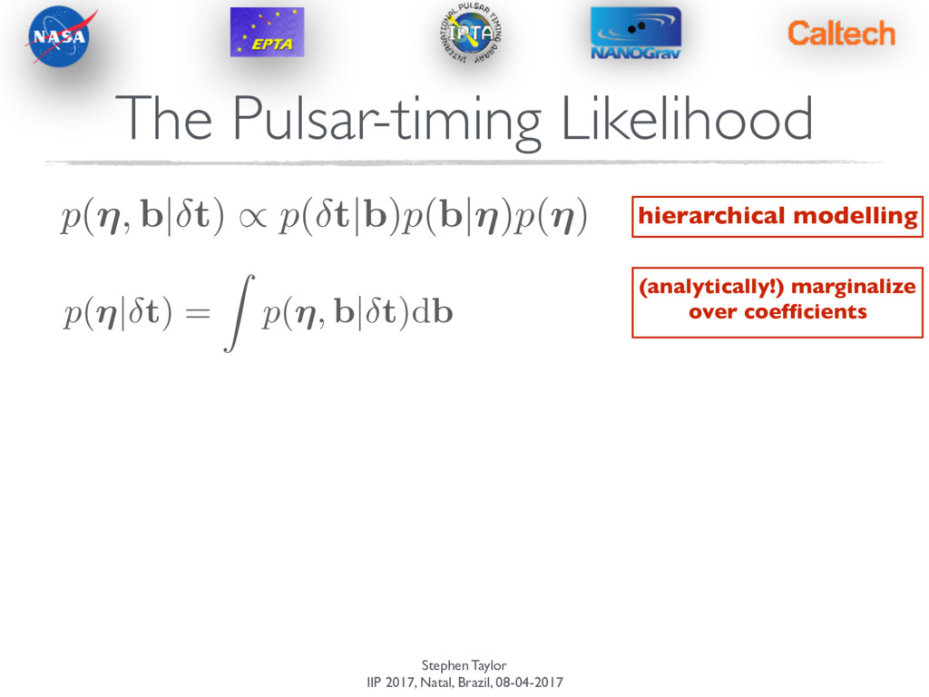
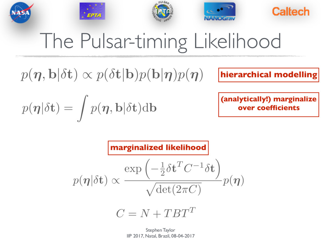
p(⌘| t) = Z p(⌘, b| t)db p(⌘, b| t) / p( t|b)p(b|⌘)p(⌘) p ( ⌘| t ) / exp ⇣ 1 2 tT C 1 t ⌘ p det(2 ⇡C ) p ( ⌘ ) C = N + TBTT hierarchical modelling (analytically!) marginalize over coefficients marginalized likelihood
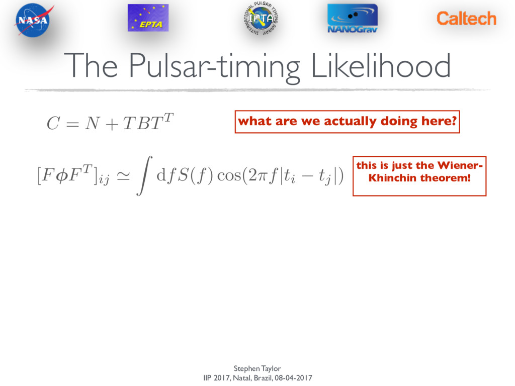
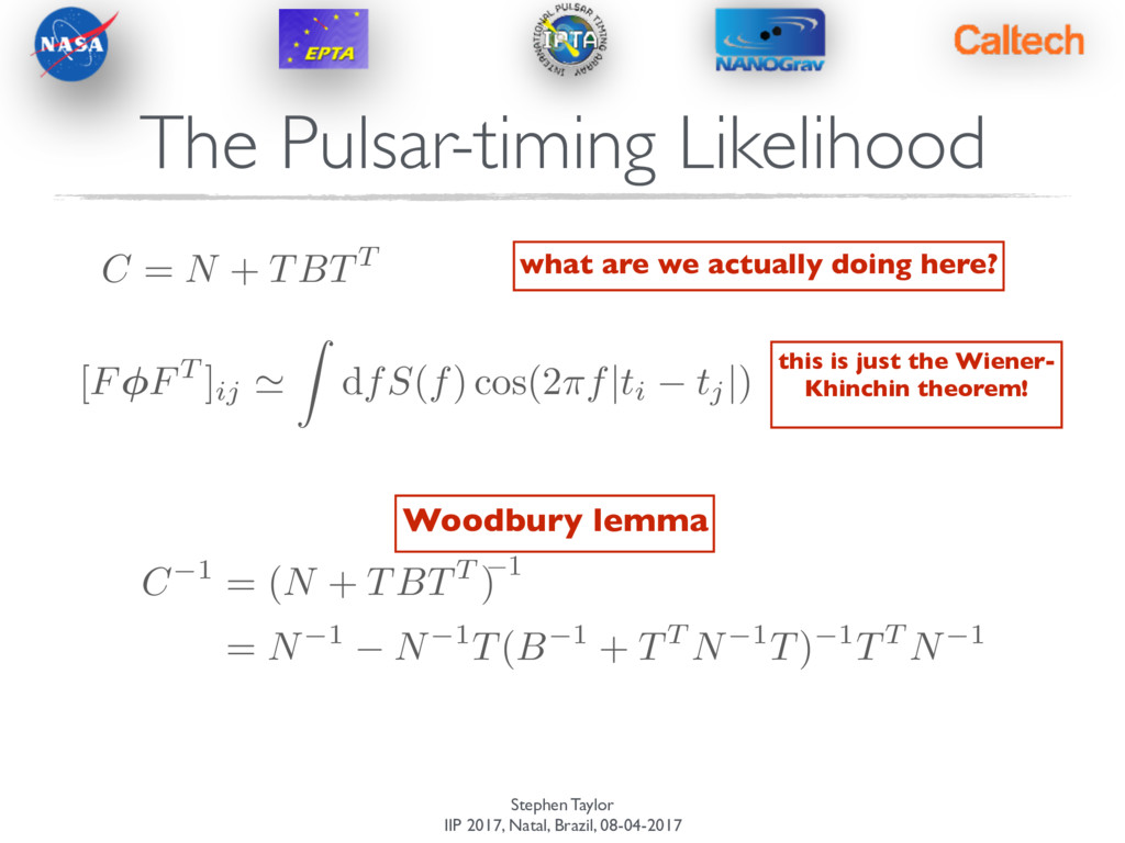
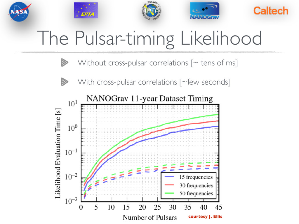
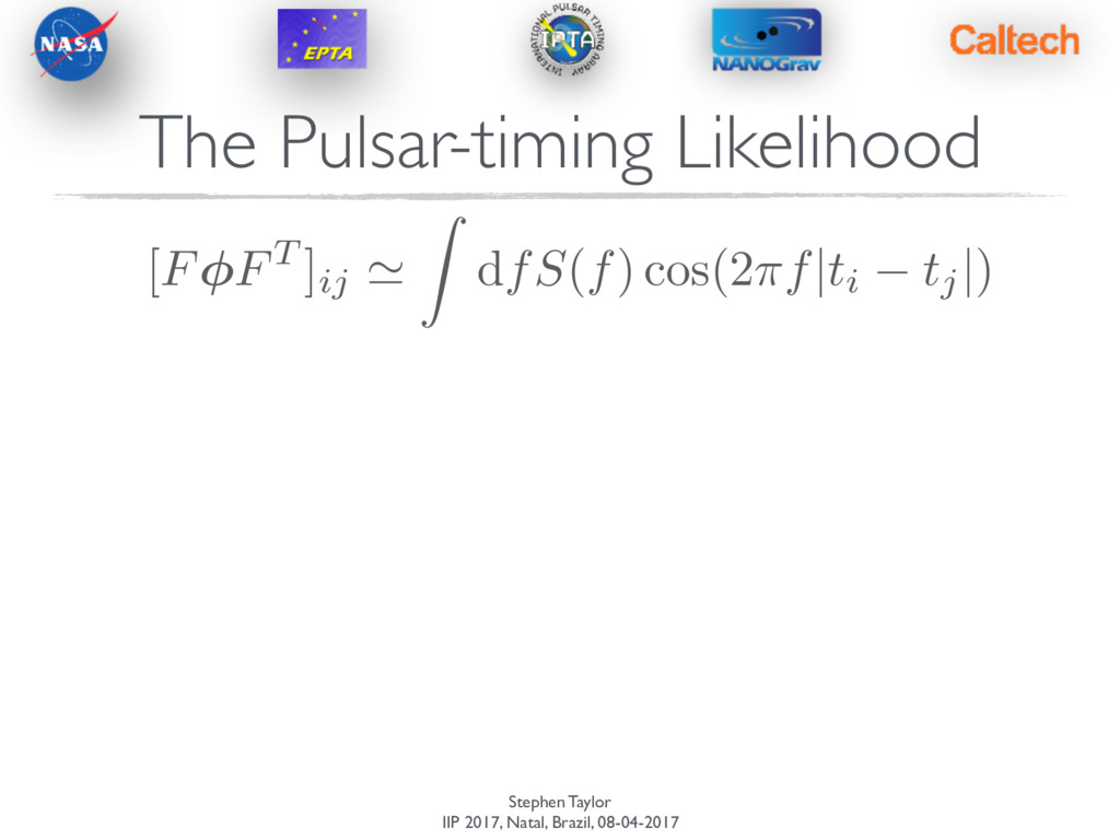
C = N + TBTT what are we actually doing here? this is just the Wiener- Khinchin theorem! [ F FT ]ij ' Z d fS ( f ) cos(2 ⇡f|ti tj | ) C 1 = (N + TBTT ) = N 1 N 1T(B 1 + TT N 1T) 1TT N 1 Woodbury lemma 1
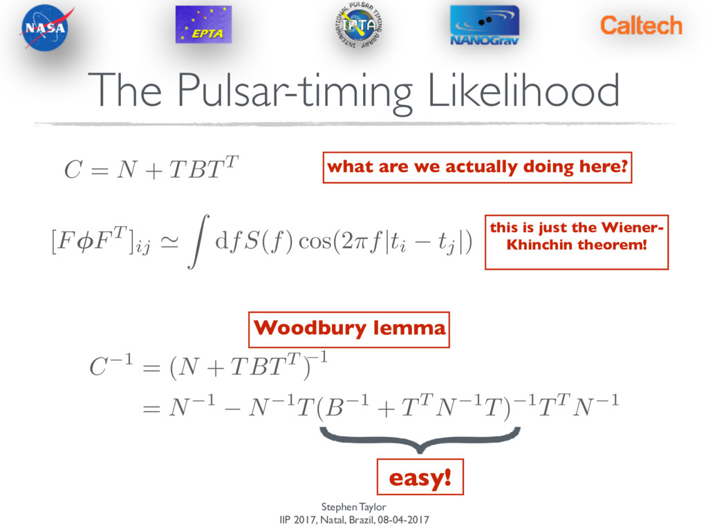
C = N + TBTT what are we actually doing here? this is just the Wiener- Khinchin theorem! [ F FT ]ij ' Z d fS ( f ) cos(2 ⇡f|ti tj | ) C 1 = (N + TBTT ) = N 1 N 1T(B 1 + TT N 1T) 1TT N 1 easy! Woodbury lemma 1
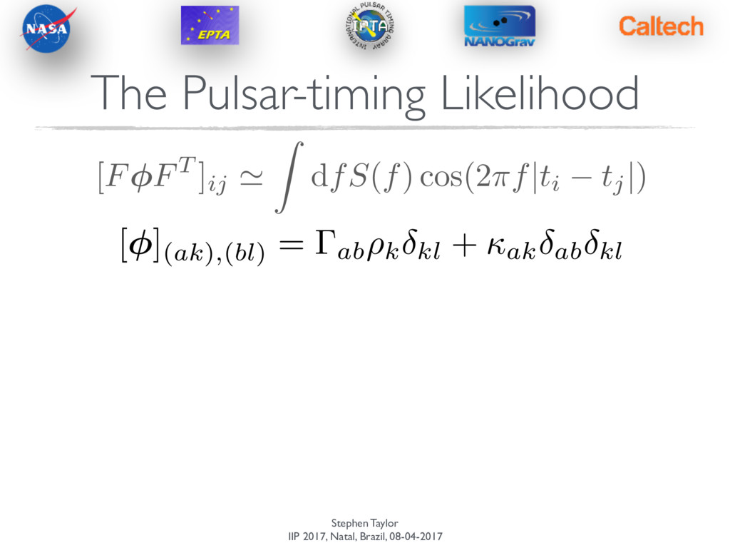
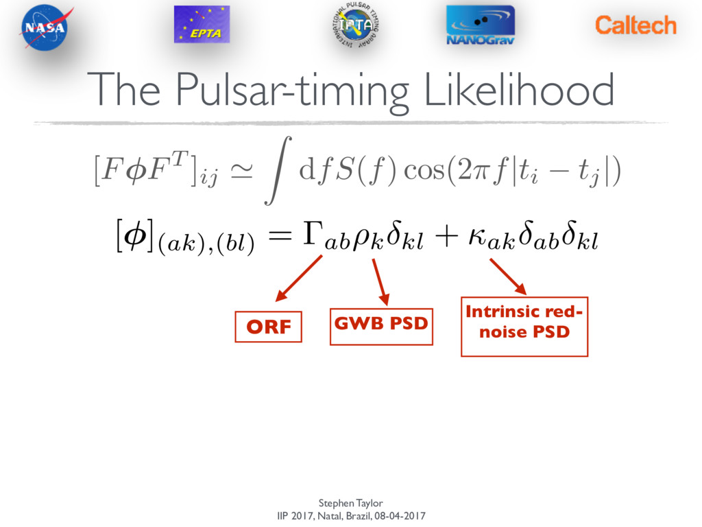
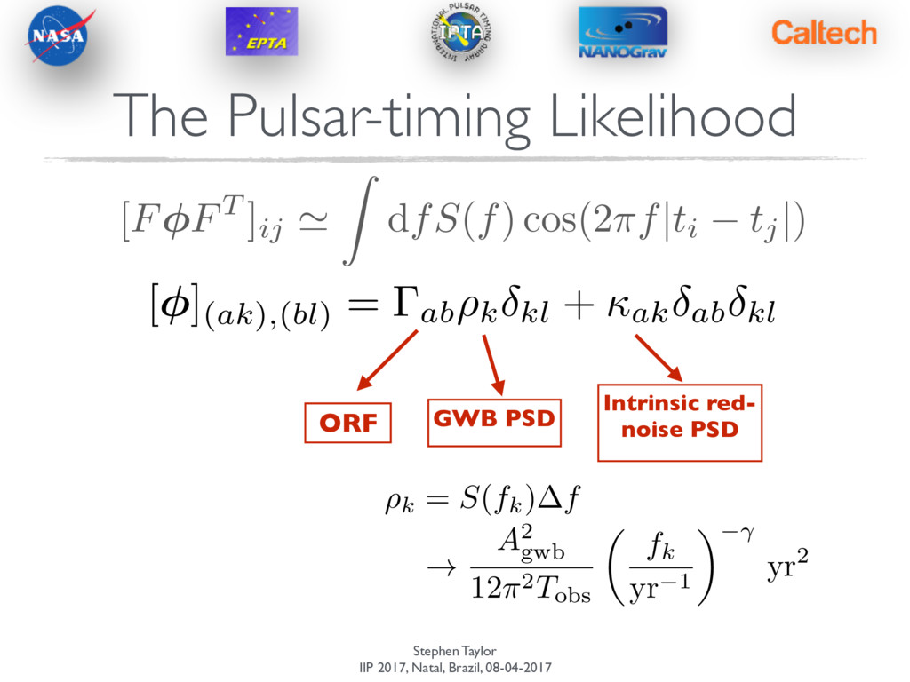
ORF GWB PSD Intrinsic red- noise PSD [ F FT ]ij ' Z d fS ( f ) cos(2 ⇡f|ti tj | ) [ ](ak),(bl) = ab⇢k kl + ak ab kl ⇢k = S(fk) f ! A2 gwb 12⇡2 T obs ✓ fk yr 1 ◆ yr2
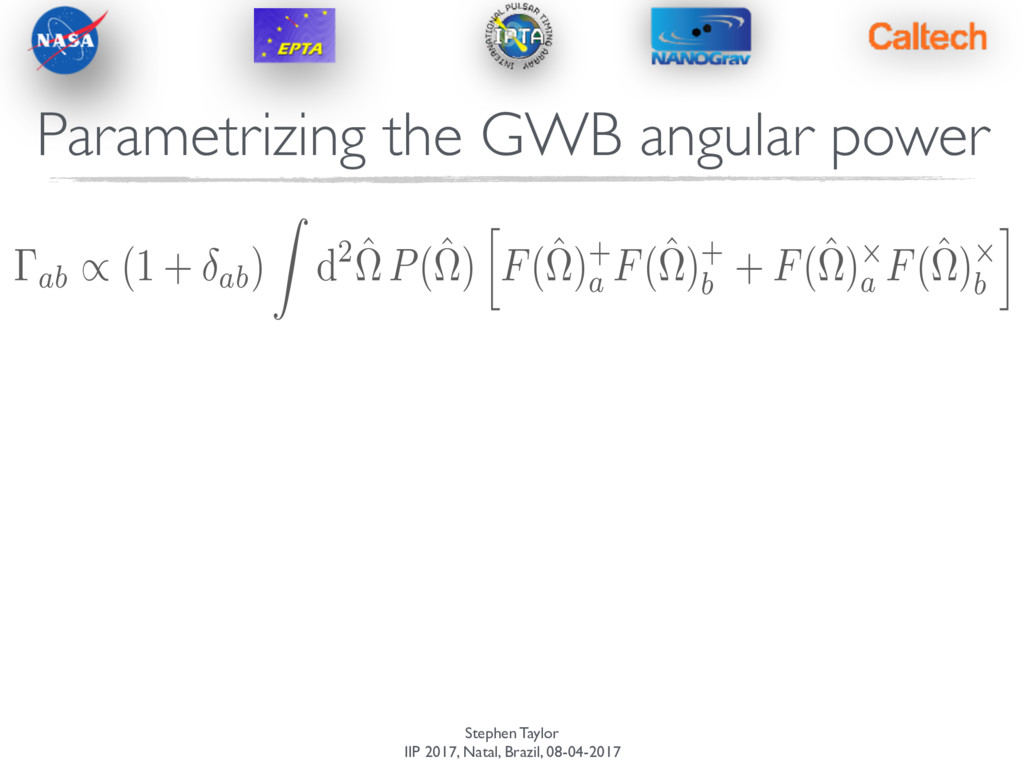
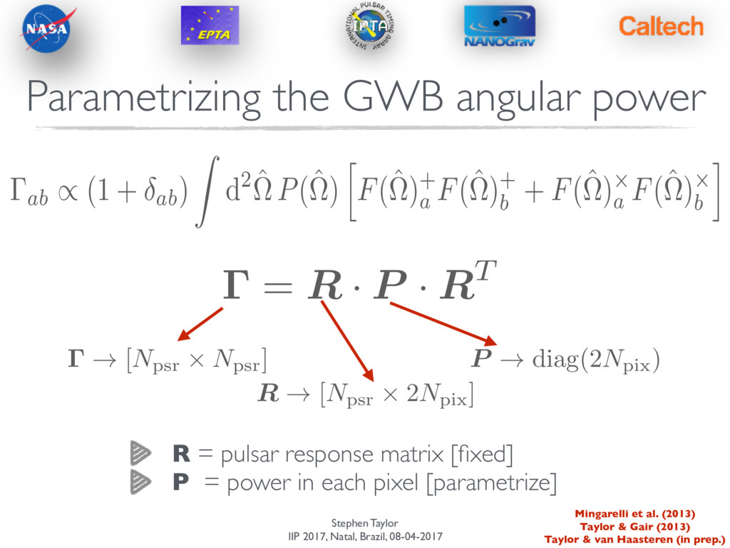
angular power ab / (1 + ab) Z d2 ˆ ⌦P(ˆ ⌦) h F(ˆ ⌦)+ a F(ˆ ⌦)+ b + F(ˆ ⌦)⇥ a F(ˆ ⌦)⇥ b i = R · P · RT R ! [N psr ⇥ 2N pix ] P ! diag(2N pix ) ! [Npsr ⇥ Npsr] R = pulsar response matrix [fixed] P = power in each pixel [parametrize] Mingarelli et al. (2013) Taylor & Gair (2013) Taylor & van Haasteren (in prep.)
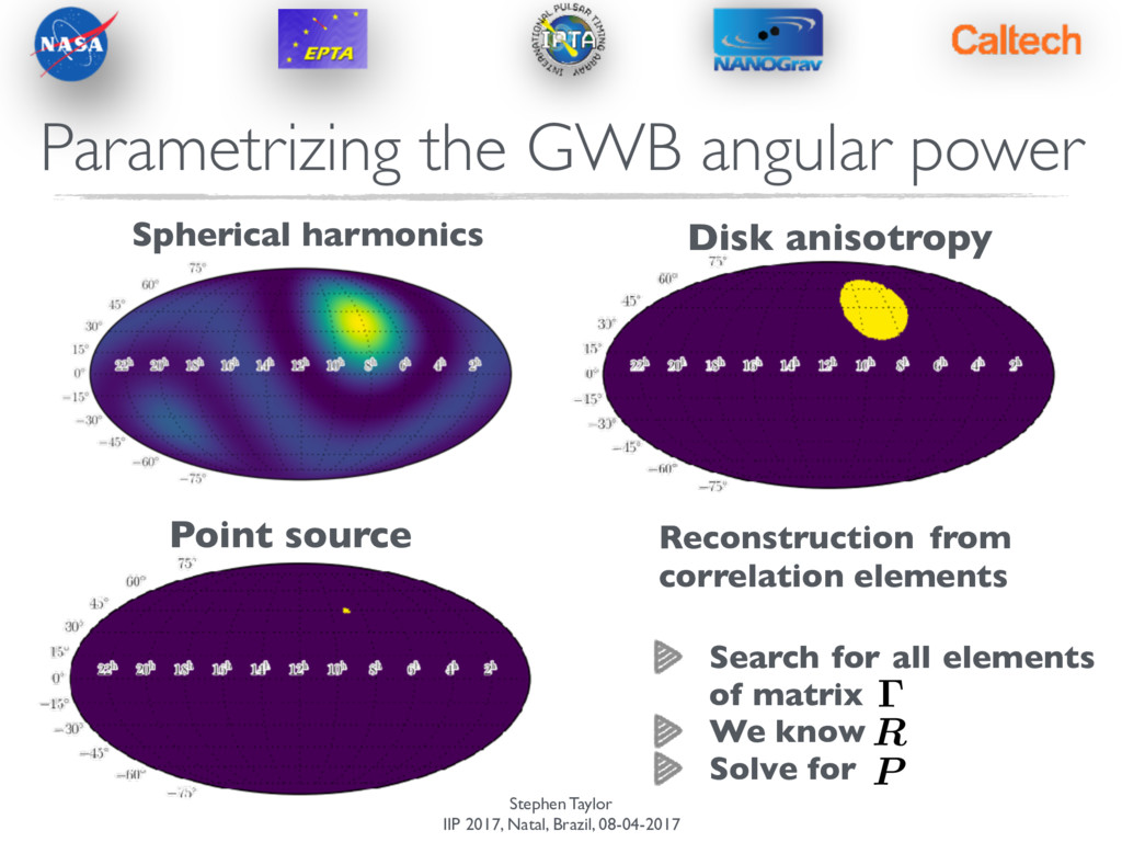
angular power Spherical harmonics Disk anisotropy Point source Reconstruction from correlation elements Search for all elements of matrix We know Solve for R P
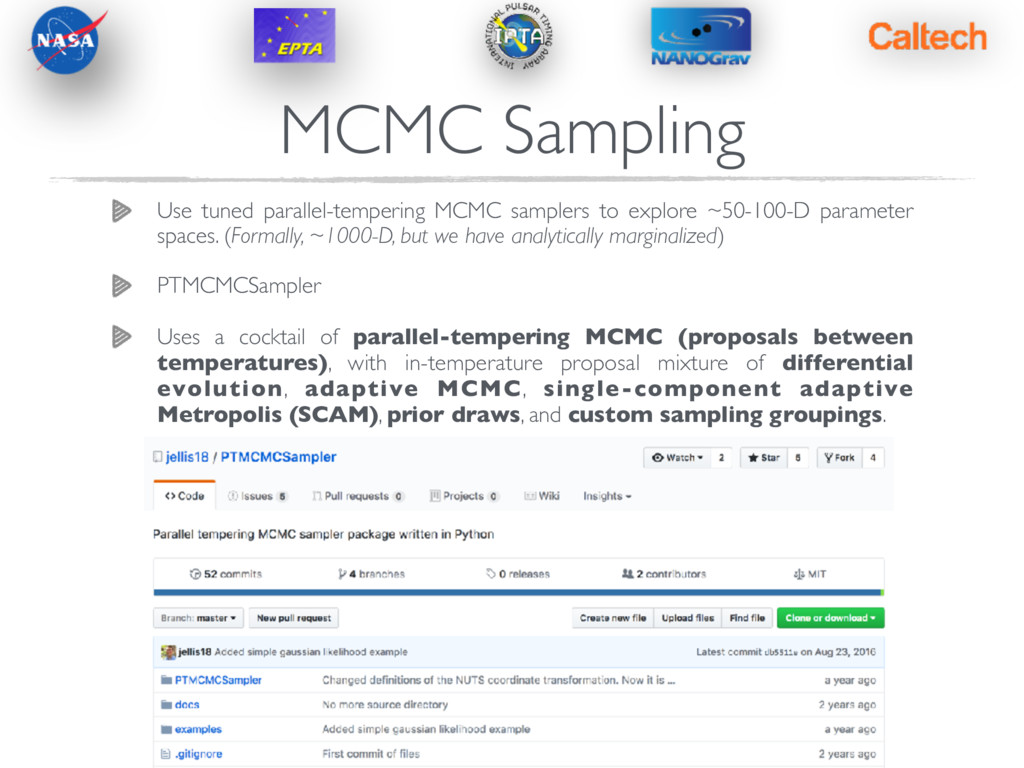
tuned parallel-tempering MCMC samplers to explore ~50-100-D parameter spaces. (Formally, ~1000-D, but we have analytically marginalized) PTMCMCSampler Uses a cocktail of parallel-tempering MCMC (proposals between temperatures), with in-temperature proposal mixture of differential evolution, adaptive MCMC, single-component adaptive Metropolis (SCAM), prior draws, and custom sampling groupings.
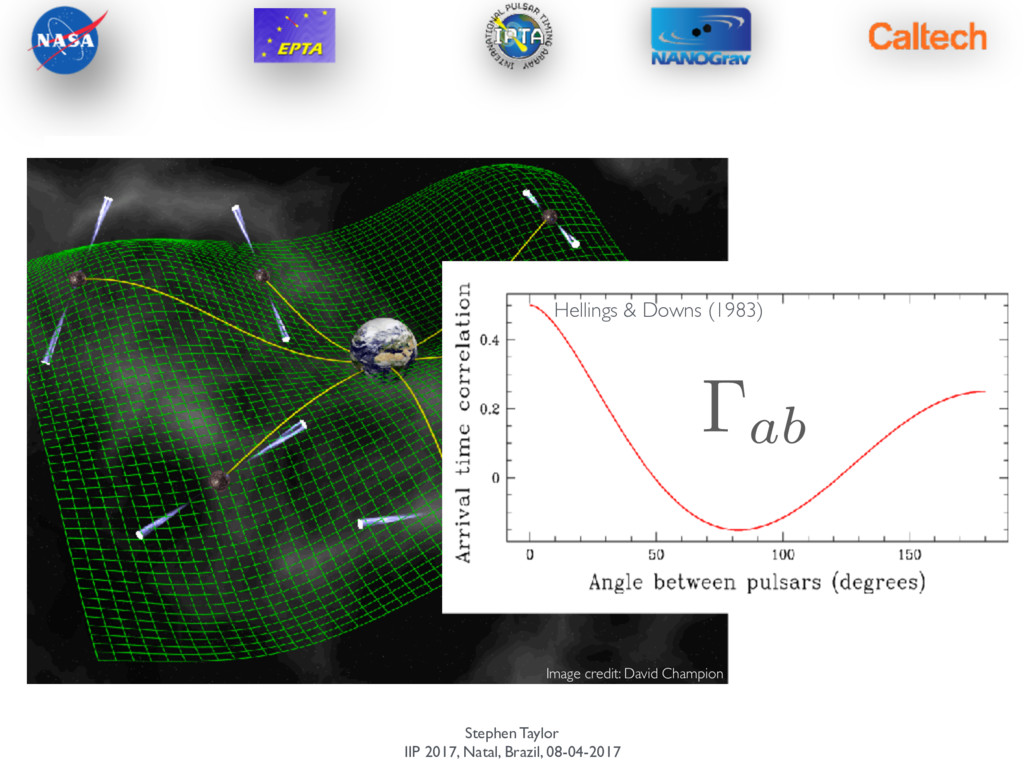
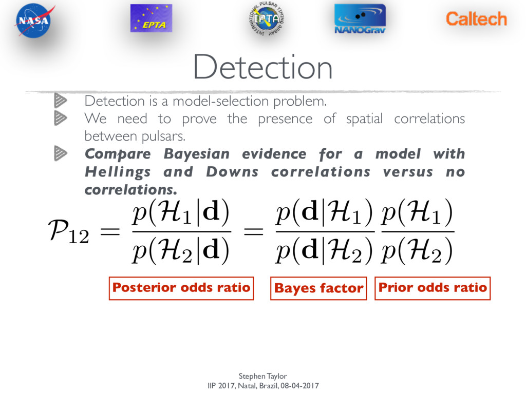
a model-selection problem. We need to prove the presence of spatial correlations between pulsars. Compare Bayesian evidence for a model with Hellings and Downs correlations versus no correlations.
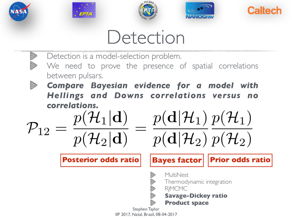
a model-selection problem. We need to prove the presence of spatial correlations between pulsars. Compare Bayesian evidence for a model with Hellings and Downs correlations versus no correlations. P12 = p(H1 |d) p(H2 |d) = p(d|H1) p(d|H2) p(H1) p(H2) Posterior odds ratio Bayes factor Prior odds ratio
a model-selection problem. We need to prove the presence of spatial correlations between pulsars. Compare Bayesian evidence for a model with Hellings and Downs correlations versus no correlations. P12 = p(H1 |d) p(H2 |d) = p(d|H1) p(d|H2) p(H1) p(H2) Posterior odds ratio Bayes factor Prior odds ratio MultiNest Thermodynamic integration RJMCMC Savage-Dickey ratio Product space
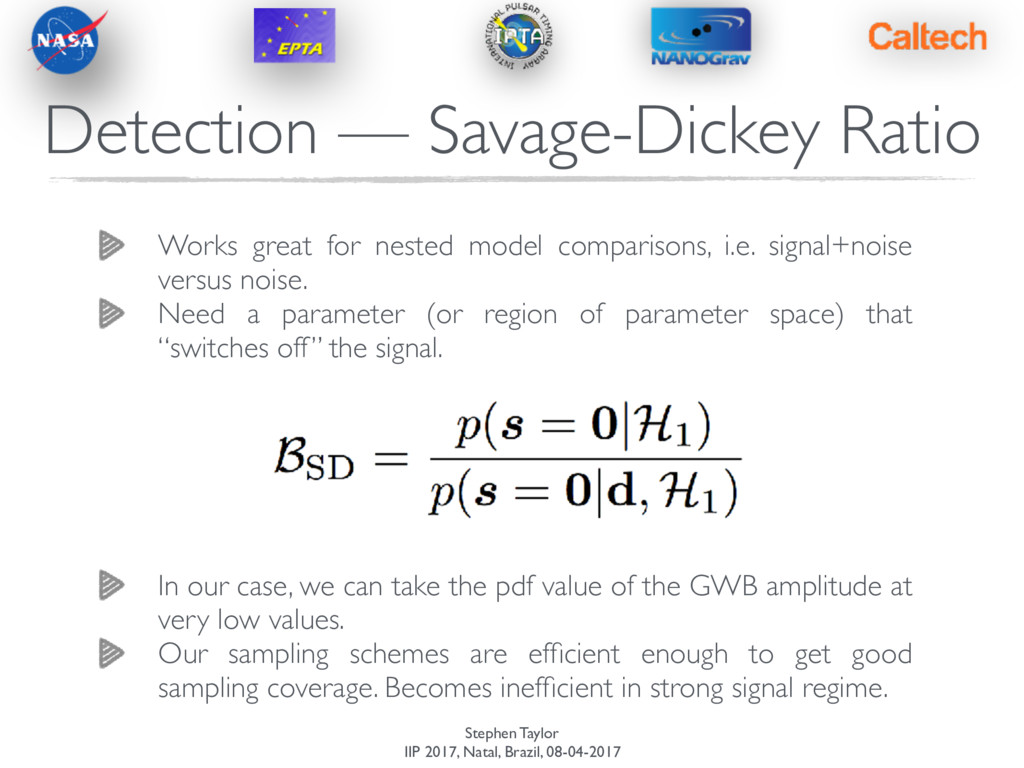
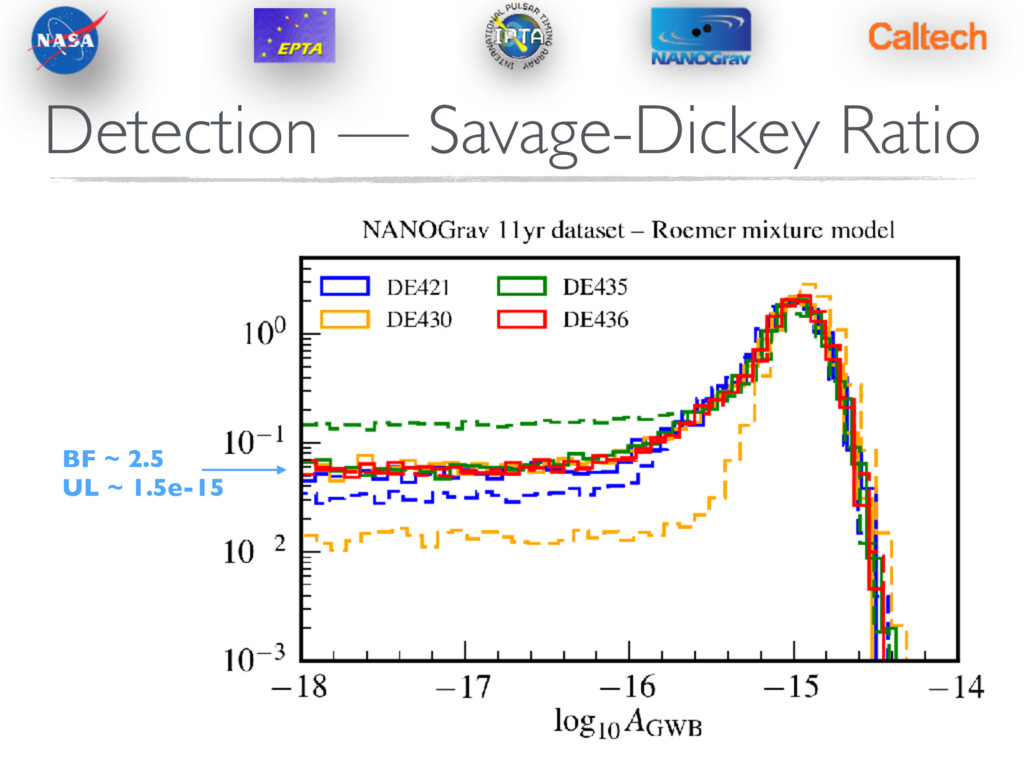
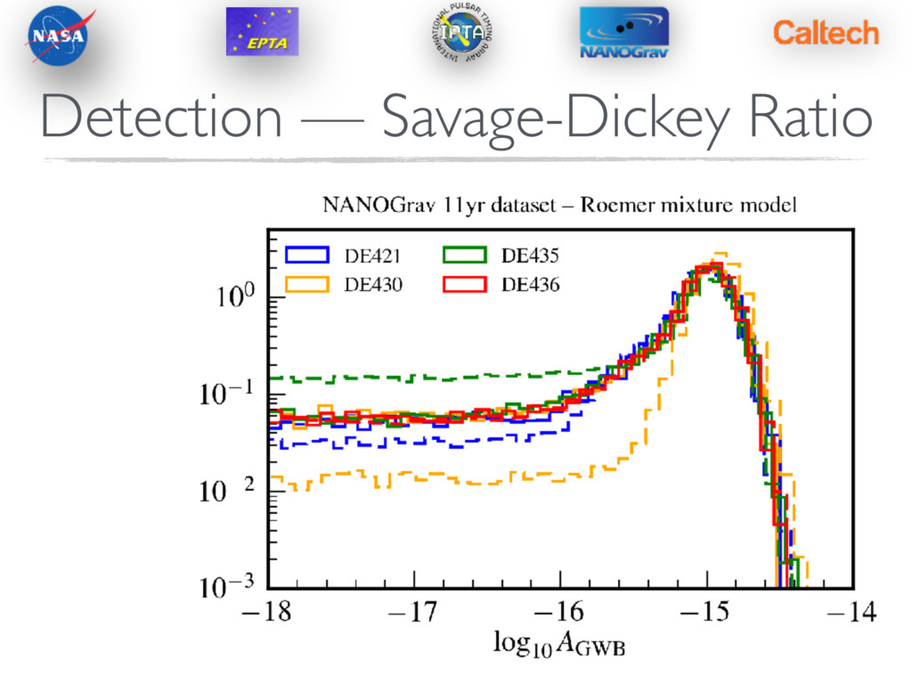
Ratio Works great for nested model comparisons, i.e. signal+noise versus noise. Need a parameter (or region of parameter space) that “switches off” the signal. In our case, we can take the pdf value of the GWB amplitude at very low values. Our sampling schemes are efficient enough to get good sampling coverage. Becomes inefficient in strong signal regime.
Method Product space sampling is ridiculously easy. [Carlin & Chib (1995), but more recently Veitch (2007, thesis), Hee et al. (2016)] Search parameters are the union of all model parameter spaces. Add a model indexing variable to parameter space. Current location of indexing variable says which likelihood is “switched on” Relative time spent at each value of model index is the posterior odds ratio.
Significance Detection statistic (whether frequentist or Bayesian) needs context. How often can noise alone produce this? Could run many noise simulations to determine p-value of measured statistic… Better to operate on real dataset.
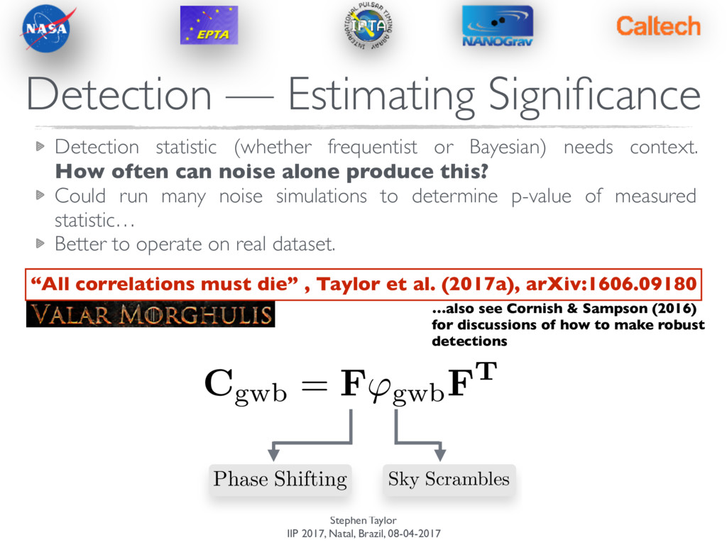
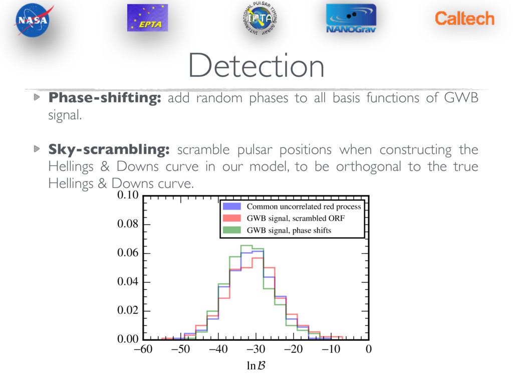
Phase Shifting Sky Scrambles …also see Cornish & Sampson (2016) for discussions of how to make robust detections Detection — Estimating Significance Detection statistic (whether frequentist or Bayesian) needs context. How often can noise alone produce this? Could run many noise simulations to determine p-value of measured statistic… Better to operate on real dataset. “All correlations must die” , Taylor et al. (2017a), arXiv:1606.09180
-40 -30 -20 -10 0 lnB 0.00 0.02 0.04 0.06 0.08 0.10 Common uncorrelated red process GWB signal, scrambled ORF GWB signal, phase shifts Phase-shifting: add random phases to all basis functions of GWB signal. Sky-scrambling: scramble pulsar positions when constructing the Hellings & Downs curve in our model, to be orthogonal to the true Hellings & Downs curve.
techniques use sophisticated hierarchical modeling and MCMC strategies to search for correlations. Bayes factors are now quite cheap to compute. [Savage-Dickey, Product-space sampling] Phase-shifting and sky-scrambling give context to these Bayes factors. [“All correlations must die”, arXiv:1606.09180] We can also build physically-sophisticated spectral models by training Gaussian Processes on populations of binaries. Sometimes its easier to simulate the Universe than write down an equation. [Taylor et al. (2017b), arXiv:1612.02817]