2017 California Institute of Technology. Government sponsorship acknowledged Stephen R. Taylor GW Constraints On Disc Migration Via Pulsar Timing JET PROPULSION LABORATORY, CALIFORNIA INSTITUTE OF TECHNOLOGY
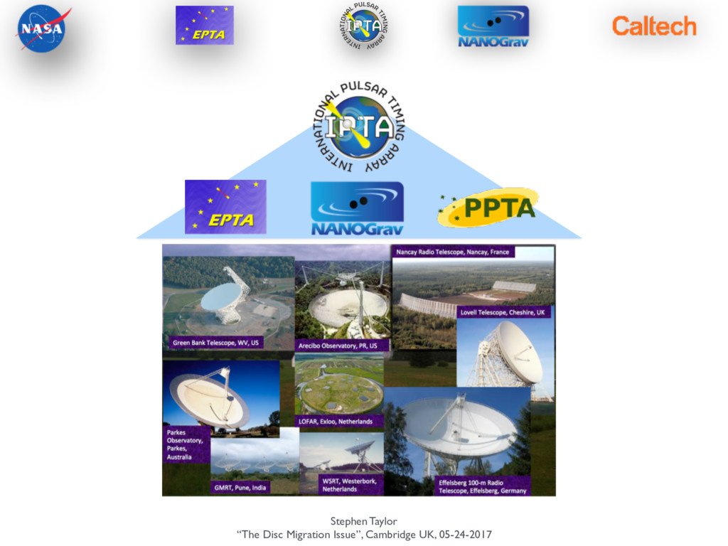
Pulsars, and precision timing Searching for gravitational waves Supermassive black-hole binaries as sources of nanohertz gravitational waves Impact of binary environmental couplings on GW signals Pulsar-timing constraints on binary environments
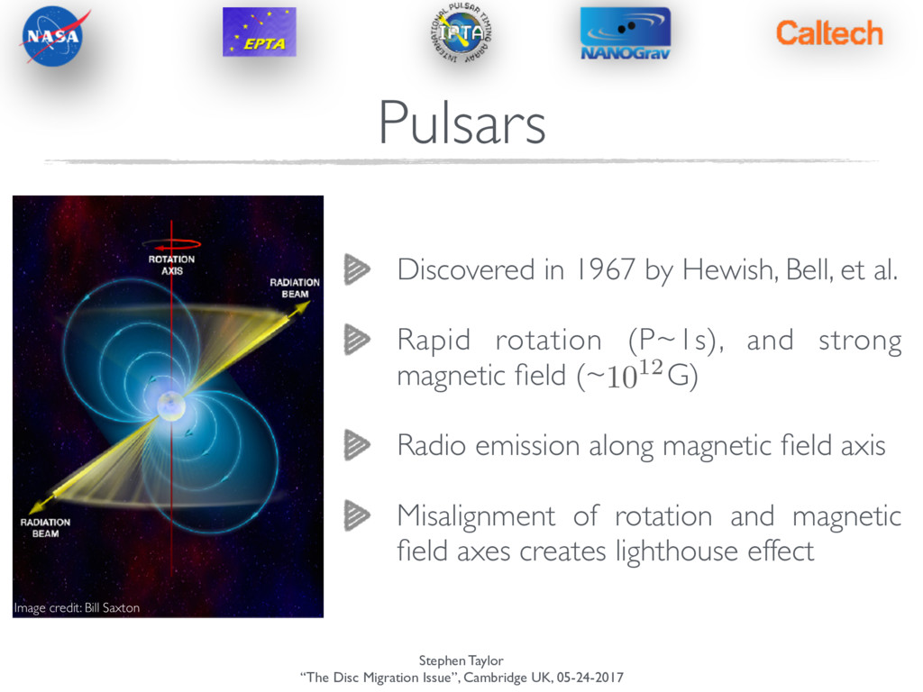
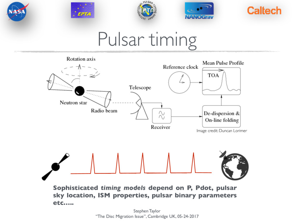
in 1967 by Hewish, Bell, et al. Rapid rotation (P~1s), and strong magnetic field (~ G) Radio emission along magnetic field axis Misalignment of rotation and magnetic field axes creates lighthouse effect 1012 Image credit: Bill Saxton Pulsars
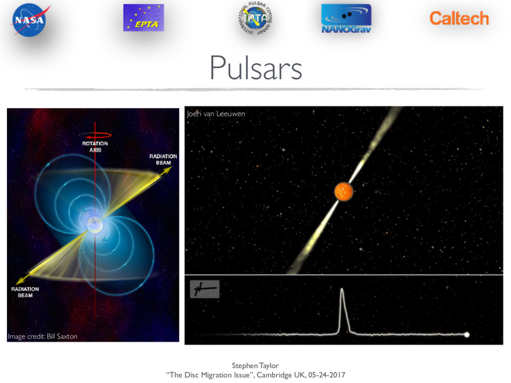
in 1967 by Hewish, Bell, et al. Rapid rotation (P~1s), and strong magnetic field (~ G) Radio emission along magnetic field axis Misalignment of rotation and magnetic field axes creates lighthouse effect 1012 Image credit: Bill Saxton Joeri van Leeuwen Pulsars
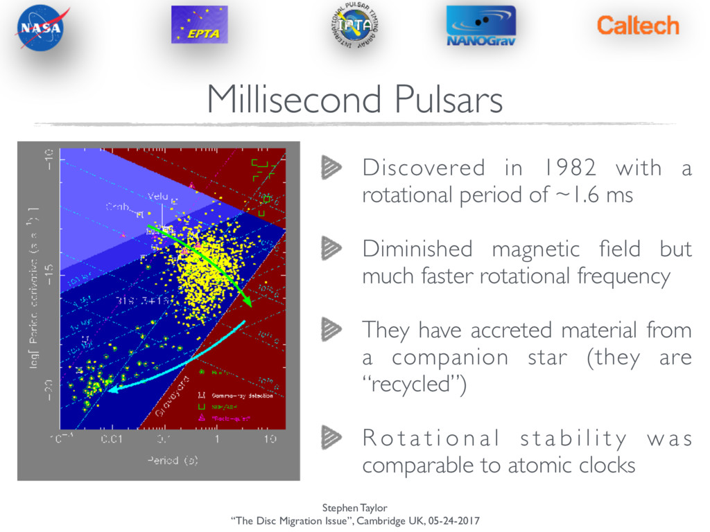
Pulsars Discovered in 1982 with a rotational period of ~1.6 ms Diminished magnetic field but much faster rotational frequency They have accreted material from a companion star (they are “recycled”) R o t a t i o n a l s t a b i l i t y w a s comparable to atomic clocks
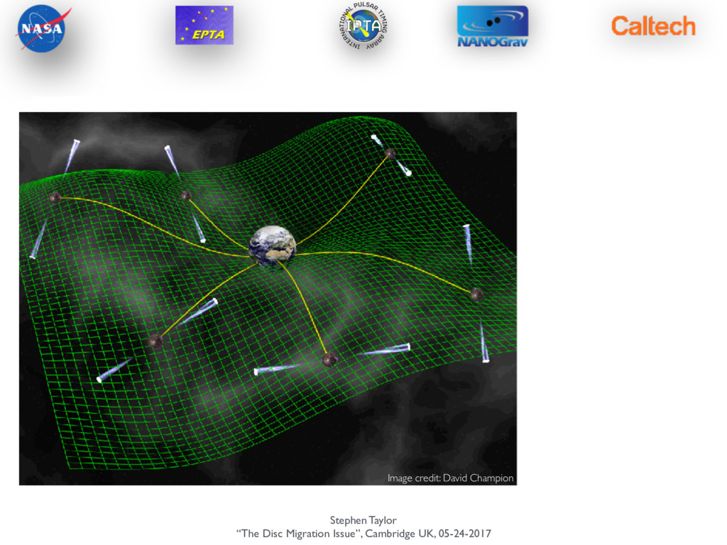
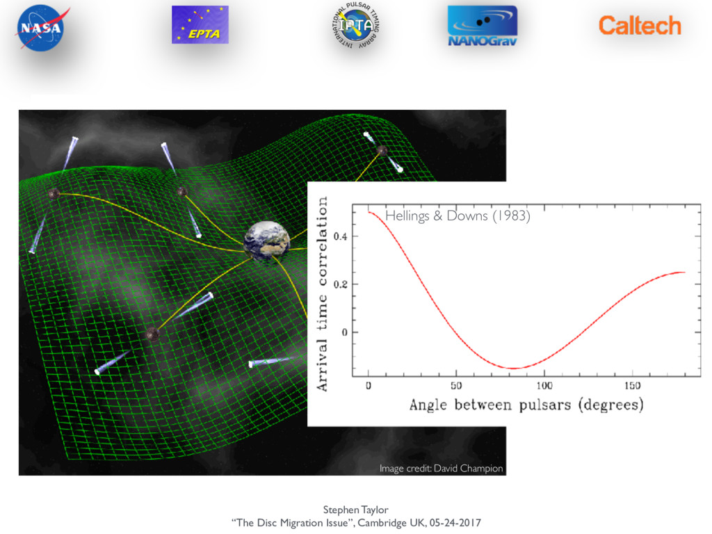
band set by total observation time (1/decades) and observational cadence (1/weeks) — [ ~ 1- 100 nHz ] Primary candidate is population of supermassive black-hole binaries Searching for GWs with pulsar timing
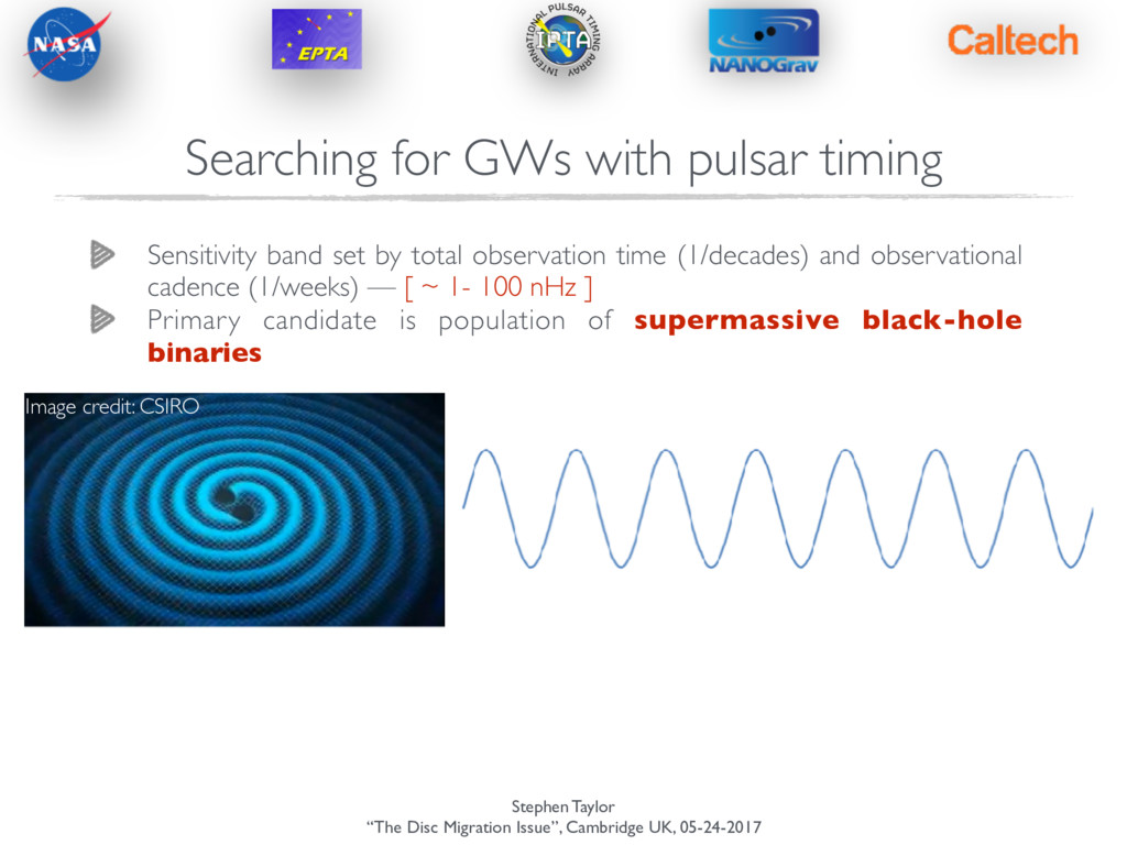
band set by total observation time (1/decades) and observational cadence (1/weeks) — [ ~ 1- 100 nHz ] Primary candidate is population of supermassive black-hole binaries Image credit: CSIRO Searching for GWs with pulsar timing
band set by total observation time (1/decades) and observational cadence (1/weeks) — [ ~ 1- 100 nHz ] Primary candidate is population of supermassive black-hole binaries Image credit: CSIRO Searching for GWs with pulsar timing
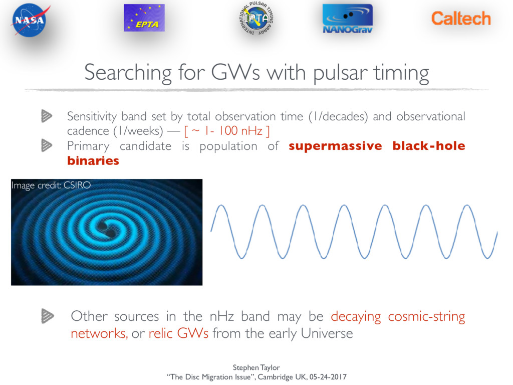
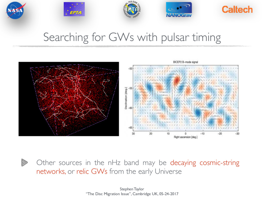
band set by total observation time (1/decades) and observational cadence (1/weeks) — [ ~ 1- 100 nHz ] Primary candidate is population of supermassive black-hole binaries Image credit: CSIRO Searching for GWs with pulsar timing Other sources in the nHz band may be decaying cosmic-string networks, or relic GWs from the early Universe
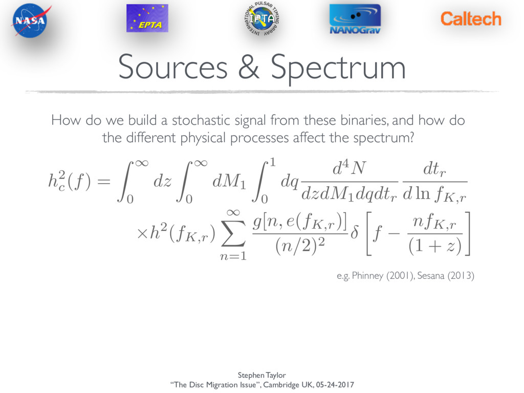
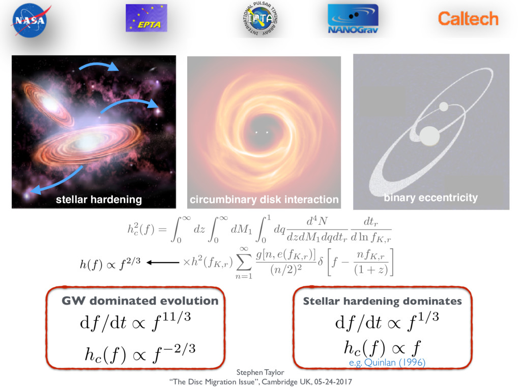
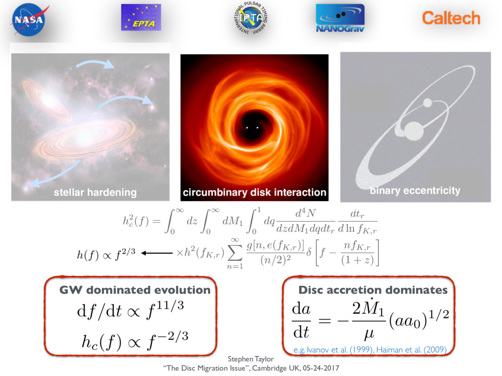
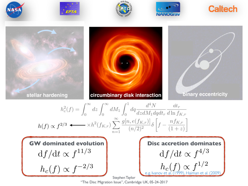
& Spectrum How do we build a stochastic signal from these binaries, and how do the different physical processes affect the spectrum? h2 c (f) = Z 1 0 dz Z 1 0 dM1 Z 1 0 dq d4N dzdM1dqdtr dtr d ln fK,r ⇥h2(fK,r) 1 X n=1 g[n, e(fK,r)] (n/2)2 f nfK,r (1 + z) e.g. Phinney (2001), Sesana (2013)
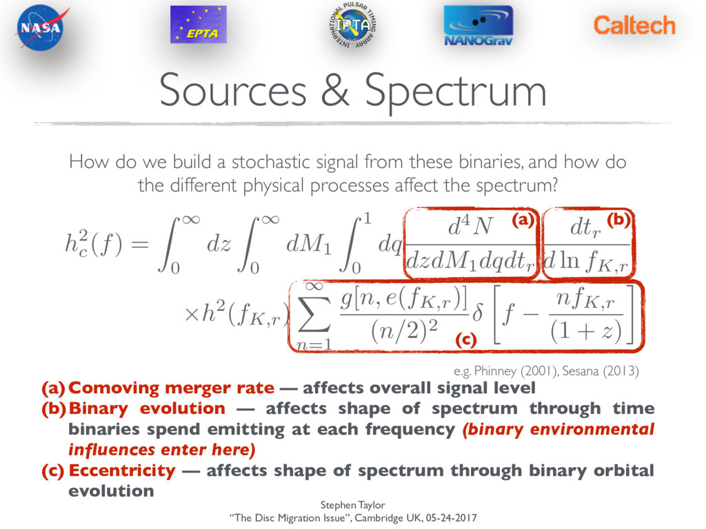
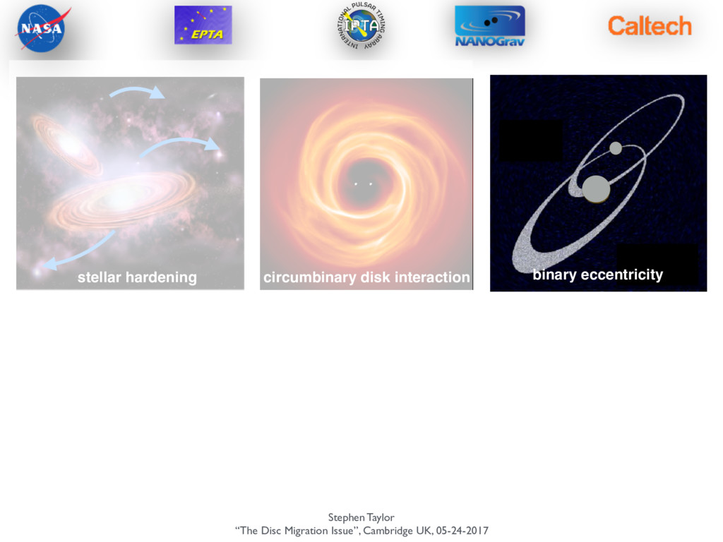
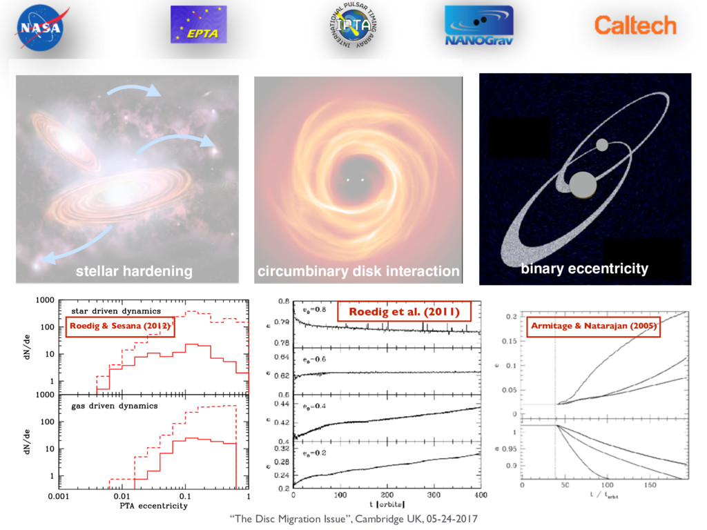
& Spectrum How do we build a stochastic signal from these binaries, and how do the different physical processes affect the spectrum? h2 c (f) = Z 1 0 dz Z 1 0 dM1 Z 1 0 dq d4N dzdM1dqdtr dtr d ln fK,r ⇥h2(fK,r) 1 X n=1 g[n, e(fK,r)] (n/2)2 f nfK,r (1 + z) e.g. Phinney (2001), Sesana (2013) (a) (b) (c) (a) Comoving merger rate — affects overall signal level (b)Binary evolution — affects shape of spectrum through time binaries spend emitting at each frequency (binary environmental influences enter here) (c) Eccentricity — affects shape of spectrum through binary orbital evolution
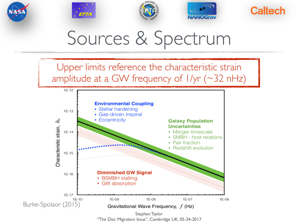
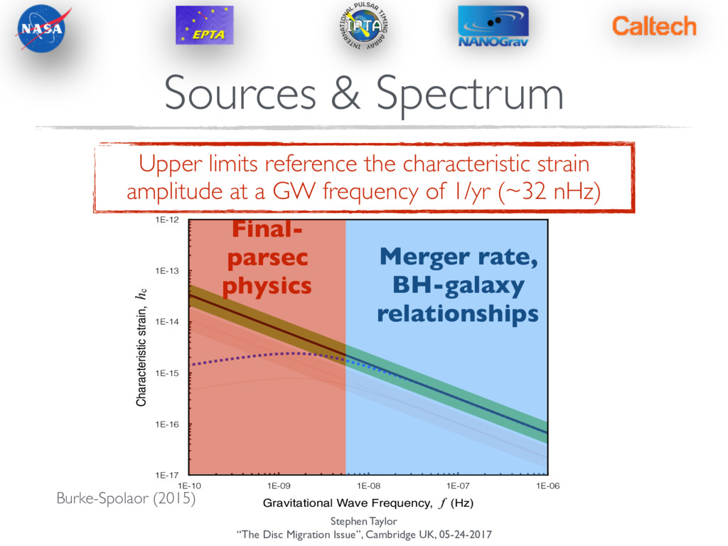
limits reference the characteristic strain amplitude at a GW frequency of 1/yr (~32 nHz) . 3.0 ⇥ 10 15 Environmental Coupling • Stellar hardening • Gas-driven inspiral • Eccentricity Galaxy Population Uncertainties • Merger timescale • SMBH - host relations • Pair fraction • Redshift evolution Diminished GW Signal • BSMBH stalling • GW absorption Characteristic strain, hc 1E-17 1E-16 1E-15 1E-14 1E-13 1E-12 Gravitational Wave Frequency, f (Hz) 1E-10 1E-09 1E-08 1E-07 1E-06 hc f 10.— A conceptual view of how various uncertainties in the BSMBH population and the GWs we can Burke-Spolaor (2015) Sources & Spectrum
limits reference the characteristic strain amplitude at a GW frequency of 1/yr (~32 nHz) . 3.0 ⇥ 10 15 Environmental Coupling • Stellar hardening • Gas-driven inspiral • Eccentricity Galaxy Population Uncertainties • Merger timescale • SMBH - host relations • Pair fraction • Redshift evolution Diminished GW Signal • BSMBH stalling • GW absorption Characteristic strain, hc 1E-17 1E-16 1E-15 1E-14 1E-13 1E-12 Gravitational Wave Frequency, f (Hz) 1E-10 1E-09 1E-08 1E-07 1E-06 hc f 10.— A conceptual view of how various uncertainties in the BSMBH population and the GWs we can Final- parsec physics Merger rate, BH-galaxy relationships Burke-Spolaor (2015) Sources & Spectrum
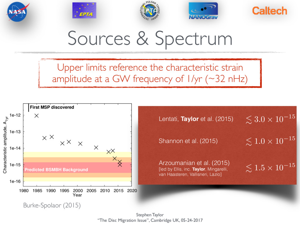
Taylor et al. (2015) Shannon et al. (2015) Arzoumanian et al. (2015) [led by Ellis, inc. Taylor, Mingarelli, van Haasteren, Vallisneri, Lazio] Upper limits reference the characteristic strain amplitude at a GW frequency of 1/yr (~32 nHz) . 1.5 ⇥ 10 15 . 3.0 ⇥ 10 15 . 1.0 ⇥ 10 15 Characteristic amplitude, A1yr Year First MSP discovered 1e-16 1e-15 1e-14 1e-13 1e-12 1980 1985 1990 1995 2000 2005 2010 2015 2020 Predicted BSMBH Background Fig. 5.— Upper limits on the power-law GWB for a spectral index ↵ = 2/3. Limits improved steadily after dedicated timing of millisecond pul- Burke-Spolaor (2015) Sources & Spectrum
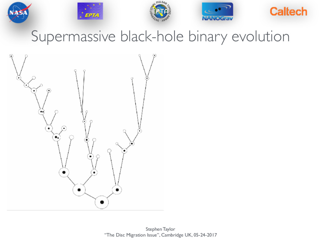
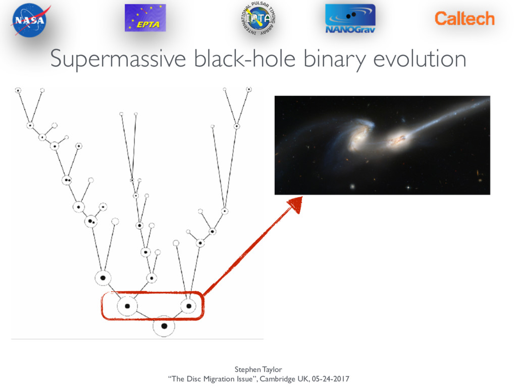
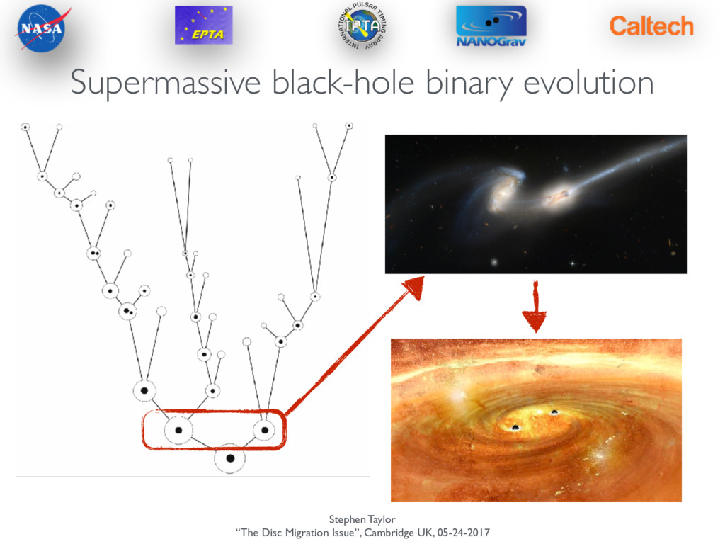
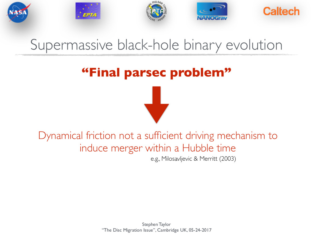
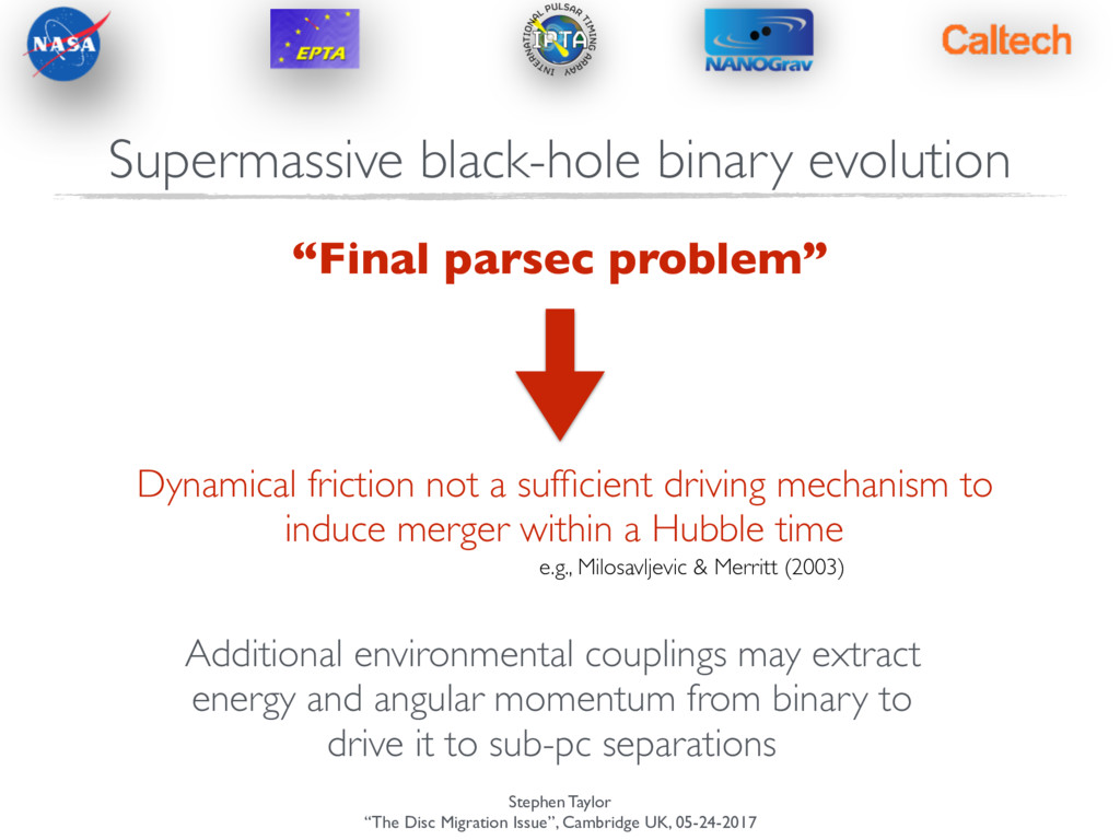
parsec problem” Dynamical friction not a sufficient driving mechanism to induce merger within a Hubble time e.g., Milosavljevic & Merritt (2003) Supermassive black-hole binary evolution
parsec problem” Dynamical friction not a sufficient driving mechanism to induce merger within a Hubble time e.g., Milosavljevic & Merritt (2003) Additional environmental couplings may extract energy and angular momentum from binary to drive it to sub-pc separations Supermassive black-hole binary evolution
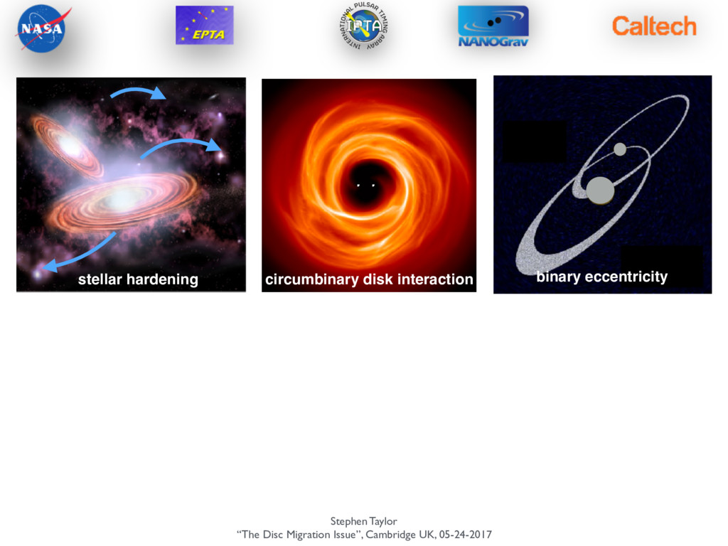
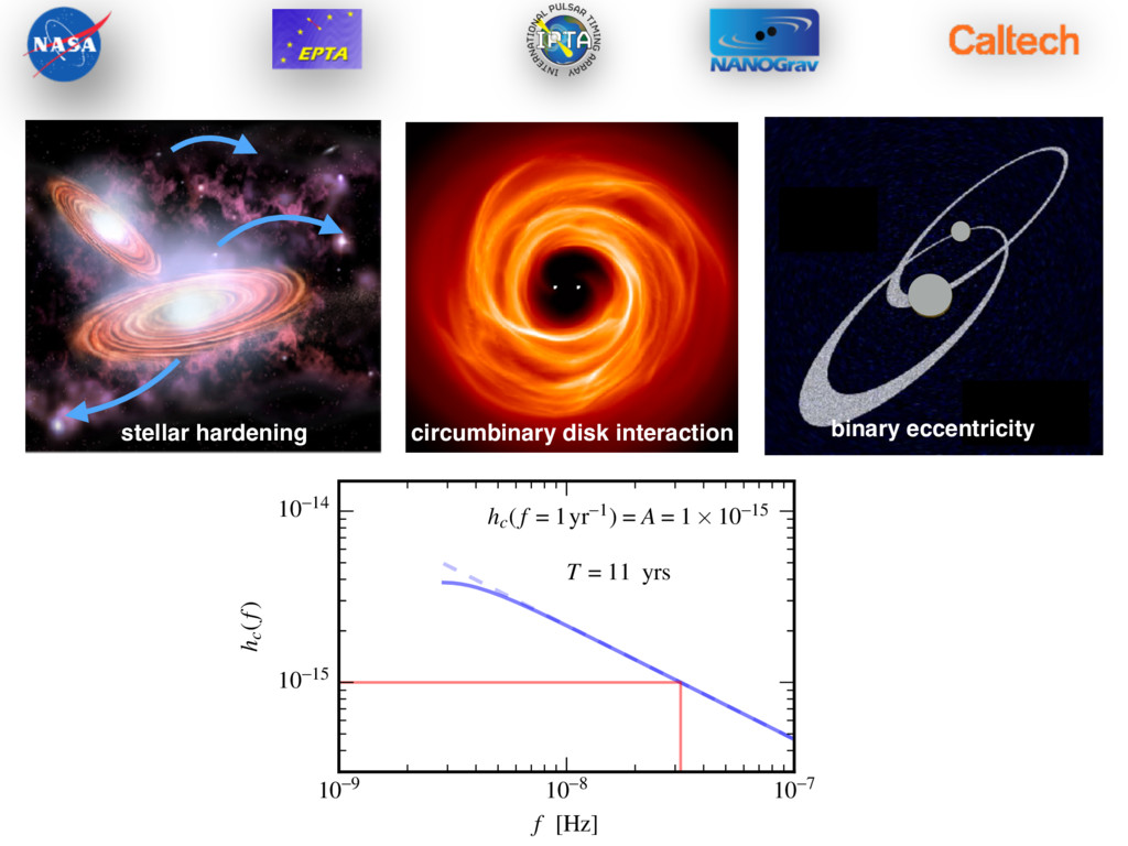
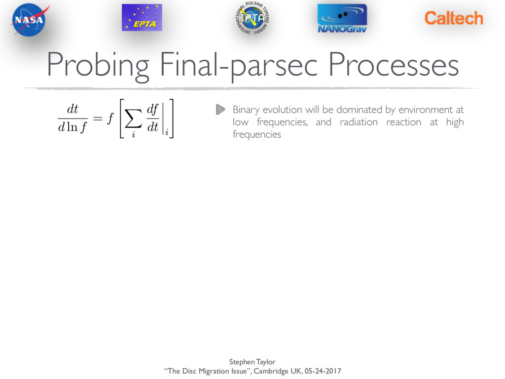
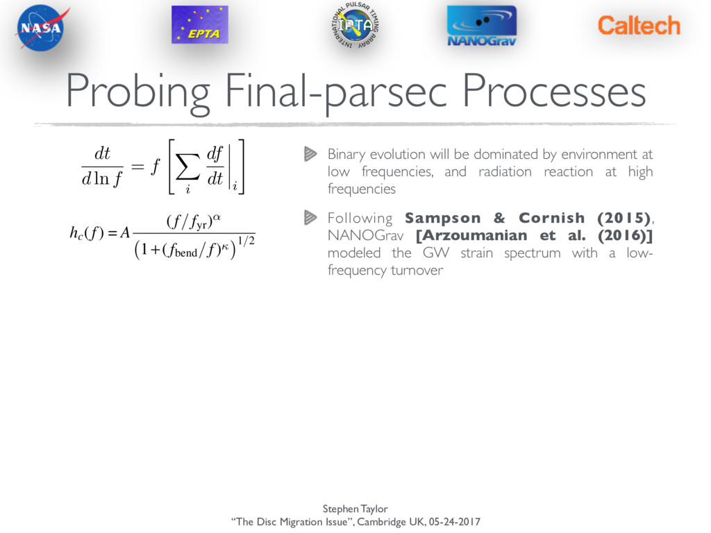
Final-parsec Processes Binary evolution will be dominated by environment at low frequencies, and radiation reaction at high frequencies dt d ln f = f " X i df dt i #
Final-parsec Processes t/d ln f term) of this equation (see Colpi 2014, for a w of SMBHB coalescence). Following Sampson et al. 5) we can generalize the frequency dependence of the n spectrum to dt d ln f = f ✓ d f dt ◆-1 = f X i ✓ d f dt ◆ i !-1 , (23) e i ranges over many physical processes that are driv- he binary to coalescence. If we restrict this sum to GW- n evolution and an unspecified physical process then the n spectrum is now hc (f) = A (f/fyr )↵ 1+(fbend/f) 1/2 , (24) Binary evolution will be dominated by environment at low frequencies, and radiation reaction at high frequencies dt d ln f = f " X i df dt i # Following Sampson & Cornish (2015), NANOGrav [Arzoumanian et al. (2016)] modeled the GW strain spectrum with a low- frequency turnover
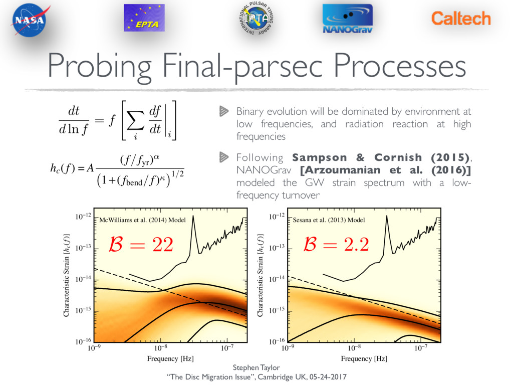
Final-parsec Processes t/d ln f term) of this equation (see Colpi 2014, for a w of SMBHB coalescence). Following Sampson et al. 5) we can generalize the frequency dependence of the n spectrum to dt d ln f = f ✓ d f dt ◆-1 = f X i ✓ d f dt ◆ i !-1 , (23) e i ranges over many physical processes that are driv- he binary to coalescence. If we restrict this sum to GW- n evolution and an unspecified physical process then the n spectrum is now hc (f) = A (f/fyr )↵ 1+(fbend/f) 1/2 , (24) Binary evolution will be dominated by environment at low frequencies, and radiation reaction at high frequencies dt d ln f = f " X i df dt i # 12 10-9 10-8 10-7 Frequency [Hz] 10-16 10-15 10-14 10-13 10-12 Characteristic Strain [hc(f)] McWilliams et al. (2014) Model 10-9 10-8 10-7 Frequency [Hz] 10-16 10-15 10-14 10-13 10-12 Characteristic Strain [hc(f)] Sesana et al. (2013) Model Figure 5. Probability density plots of the recovered GWB spectra for models A and B using the broken-power-law model parameterized by (Agw, fbend, and ) Following Sampson & Cornish (2015), NANOGrav [Arzoumanian et al. (2016)] modeled the GW strain spectrum with a low- frequency turnover B = 22 B = 2.2
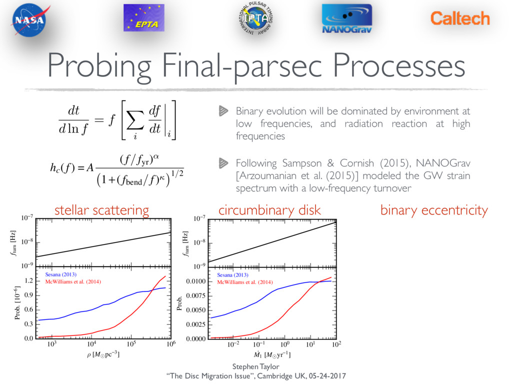
ln f term) of this equation (see Colpi 2014, for a w of SMBHB coalescence). Following Sampson et al. 5) we can generalize the frequency dependence of the n spectrum to dt d ln f = f ✓ d f dt ◆-1 = f X i ✓ d f dt ◆ i !-1 , (23) e i ranges over many physical processes that are driv- he binary to coalescence. If we restrict this sum to GW- n evolution and an unspecified physical process then the n spectrum is now hc (f) = A (f/fyr )↵ 1+(fbend/f) 1/2 , (24) Binary evolution will be dominated by environment at low frequencies, and radiation reaction at high frequencies dt d ln f = f " X i df dt i # Following Sampson & Cornish (2015), NANOGrav [Arzoumanian et al. (2015)] modeled the GW strain spectrum with a low-frequency turnover 16 10-9 10-8 10-7 fturn [Hz] 103 104 105 106 ⇢ [M pc-3] 0.0 0.3 0.6 0.9 1.2 Prob. [10-6] Sesana (2013) McWilliams et al. (2014) Figure 10. (top): Empirical mapping from fturn to ⇢ (left) and ˙ M1 (right). (bottom): Posterior distributions for the mass density of stars in the galactic core 10-9 10-8 10-7 fturn [Hz] 10-2 10-1 100 101 102 ˙ M1 [M yr-1] 0.0000 0.0025 0.0050 0.0075 0.0100 Prob. Sesana (2013) McWilliams et al. (2014) 10. (top): Empirical mapping from fturn to ⇢ (left) and ˙ M1 (right). (bottom): Posterior distributions for the mass density of stars in the galactic core stellar scattering circumbinary disk binary eccentricity Probing Final-parsec Processes
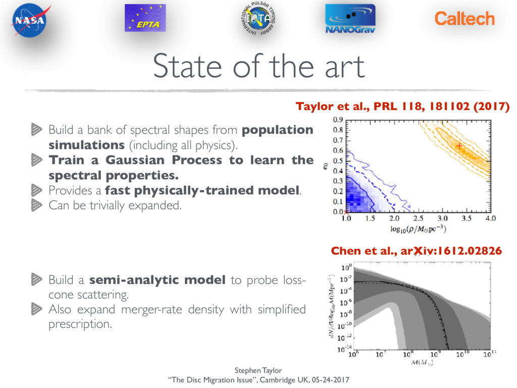
of the art Build a bank of spectral shapes from population simulations (including all physics). Train a Gaussian Process to learn the spectral properties. Provides a fast physically-trained model. Can be trivially expanded. Build a semi-analytic model to probe loss- cone scattering. Also expand merger-rate density with simplified prescription. Taylor et al., PRL 118, 181102 (2017) Chen et al., arXiv:1612.02826
Pulsar timing arrays are sensitive to nHz GWs The GW strain spectrum encodes information about SMBHB dynamical evolution Constraining the spectral shape can tell us about disc accretion, and loss-scone scattering. PTAs are expected to detect GWs within the next ~5 years.