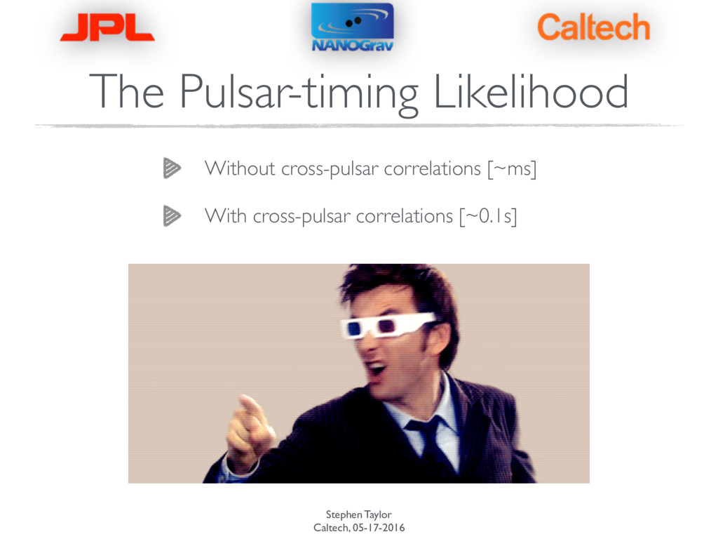
Government sponsorship acknowledged Stephen R. Taylor GRAVITATIONAL-WAVE ASTRONOMY WITH PULSAR-TIMING ARRAYS NASA POSTDOCTORAL FELLOW, JET PROPULSION LABORATORY (…really “inference strategies”)
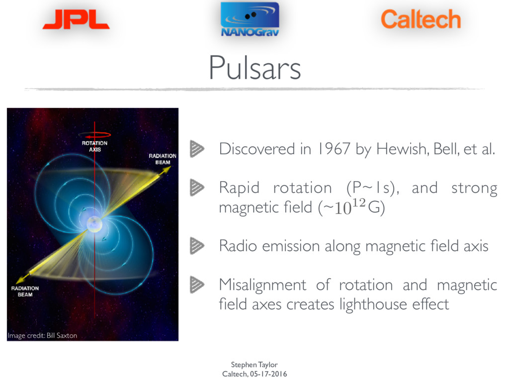
Bell, et al. Rapid rotation (P~1s), and strong magnetic field (~ G) Radio emission along magnetic field axis Misalignment of rotation and magnetic field axes creates lighthouse effect Pulsars Image credit: Bill Saxton
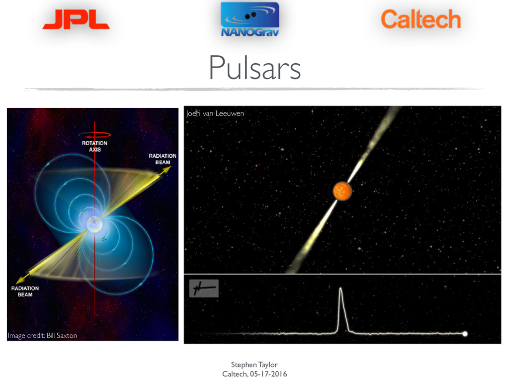
Bell, et al. Rapid rotation (P~1s), and strong magnetic field (~ G) Radio emission along magnetic field axis Misalignment of rotation and magnetic field axes creates lighthouse effect Pulsars Image credit: Bill Saxton Joeri van Leeuwen
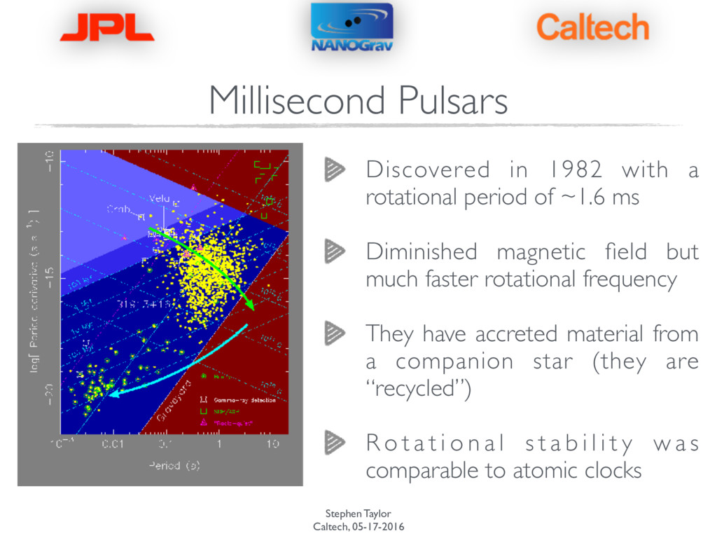
a rotational period of ~1.6 ms Diminished magnetic field but much faster rotational frequency They have accreted material from a companion star (they are “recycled”) R o t a t i o n a l s t a b i l i t y w a s comparable to atomic clocks
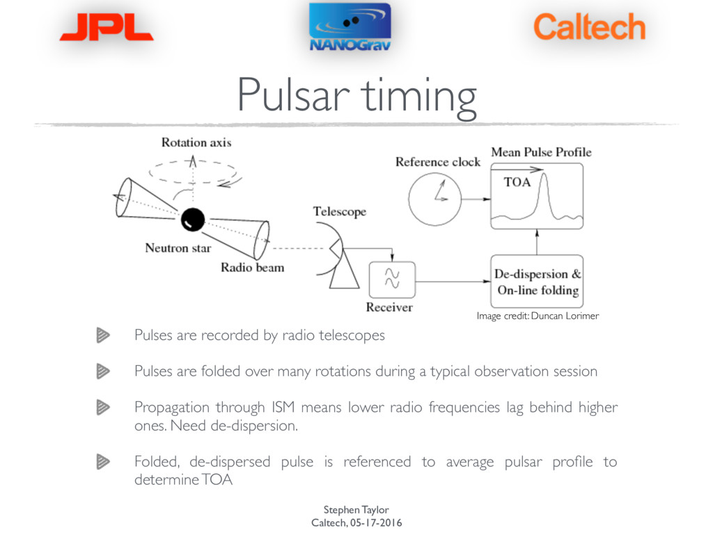
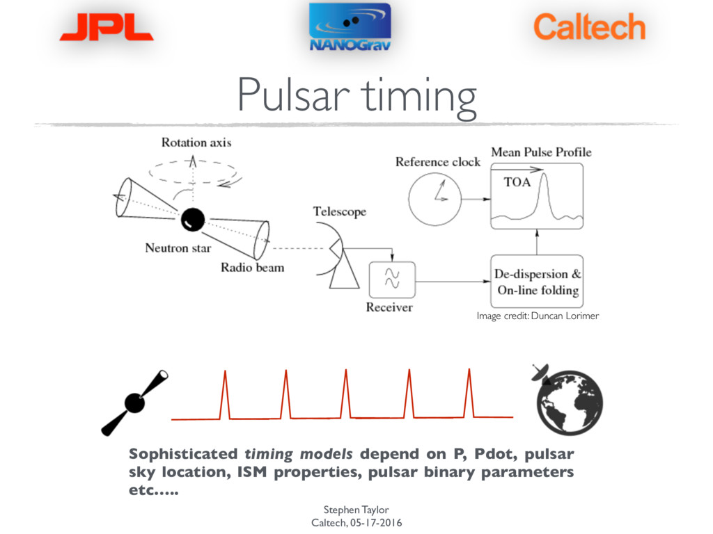
radio telescopes Pulses are folded over many rotations during a typical observation session Propagation through ISM means lower radio frequencies lag behind higher ones. Need de-dispersion. Folded, de-dispersed pulse is referenced to average pulsar profile to determine TOA Image credit: Duncan Lorimer
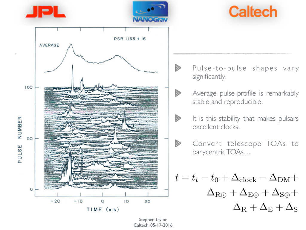
pulse-profile is remarkably stable and reproducible. It is this stability that makes pulsars excellent clocks. Conver t telescope TOAs to barycentric TOAs…
pulse-profile is remarkably stable and reproducible. It is this stability that makes pulsars excellent clocks. Conver t telescope TOAs to barycentric TOAs… t = tt t 0 + clock DM + R + E + S + R + E + S
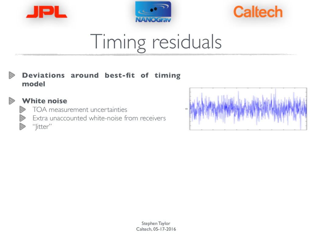
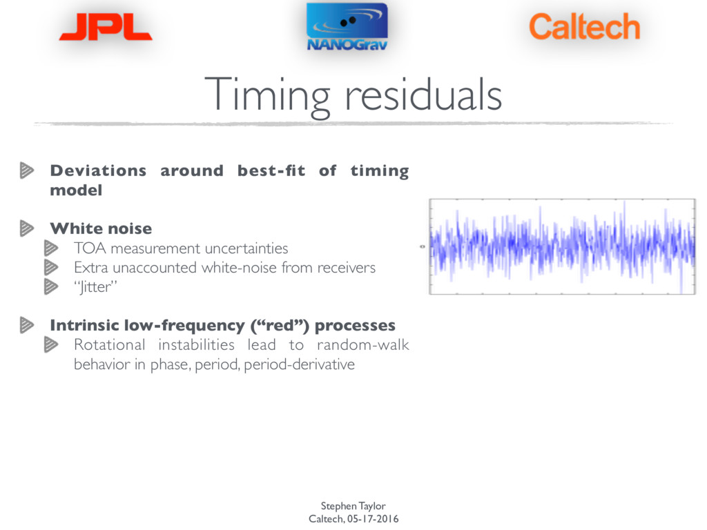
timing model White noise TOA measurement uncertainties Extra unaccounted white-noise from receivers “Jitter” Intrinsic low-frequency (“red”) processes Rotational instabilities lead to random-walk behavior in phase, period, period-derivative
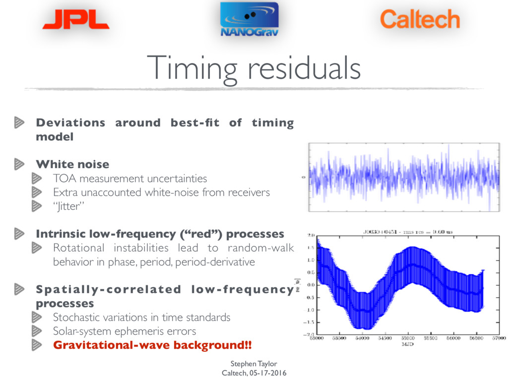
timing model White noise TOA measurement uncertainties Extra unaccounted white-noise from receivers “Jitter” Intrinsic low-frequency (“red”) processes Rotational instabilities lead to random-walk behavior in phase, period, period-derivative Spatially-correlated low-frequency processes Stochastic variations in time standards Solar-system ephemeris errors Gravitational-wave background!!
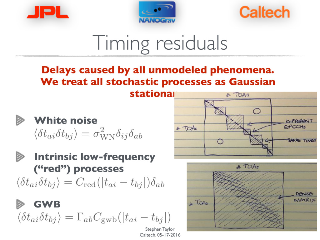
all unmodeled phenomena. We treat all stochastic processes as Gaussian stationary. White noise Intrinsic low-frequency (“red”) processes h tai tbj i = 2 WN ij ab h tai tbj i = Cred(|tai tbj |) ab h tai tbj i = abCgwb(|tai tbj |)
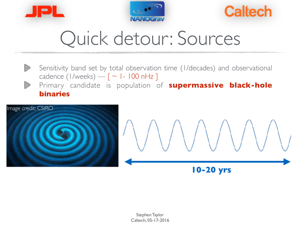
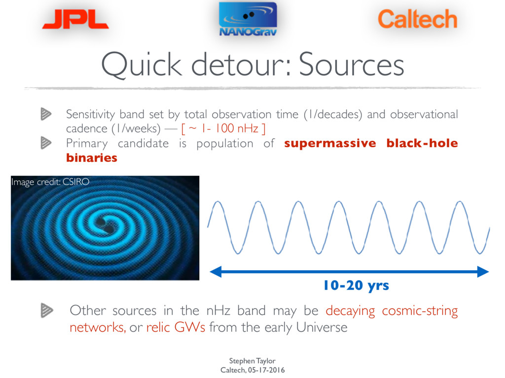
by total observation time (1/decades) and observational cadence (1/weeks) — [ ~ 1- 100 nHz ] Primary candidate is population of supermassive black-hole binaries
by total observation time (1/decades) and observational cadence (1/weeks) — [ ~ 1- 100 nHz ] Primary candidate is population of supermassive black-hole binaries Image credit: CSIRO
by total observation time (1/decades) and observational cadence (1/weeks) — [ ~ 1- 100 nHz ] Primary candidate is population of supermassive black-hole binaries Image credit: CSIRO 10-20 yrs
by total observation time (1/decades) and observational cadence (1/weeks) — [ ~ 1- 100 nHz ] Primary candidate is population of supermassive black-hole binaries Other sources in the nHz band may be decaying cosmic-string networks, or relic GWs from the early Universe Image credit: CSIRO 10-20 yrs
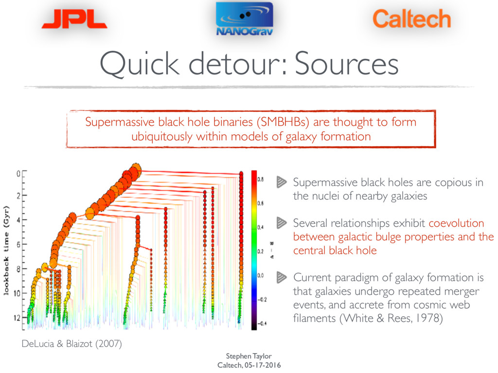
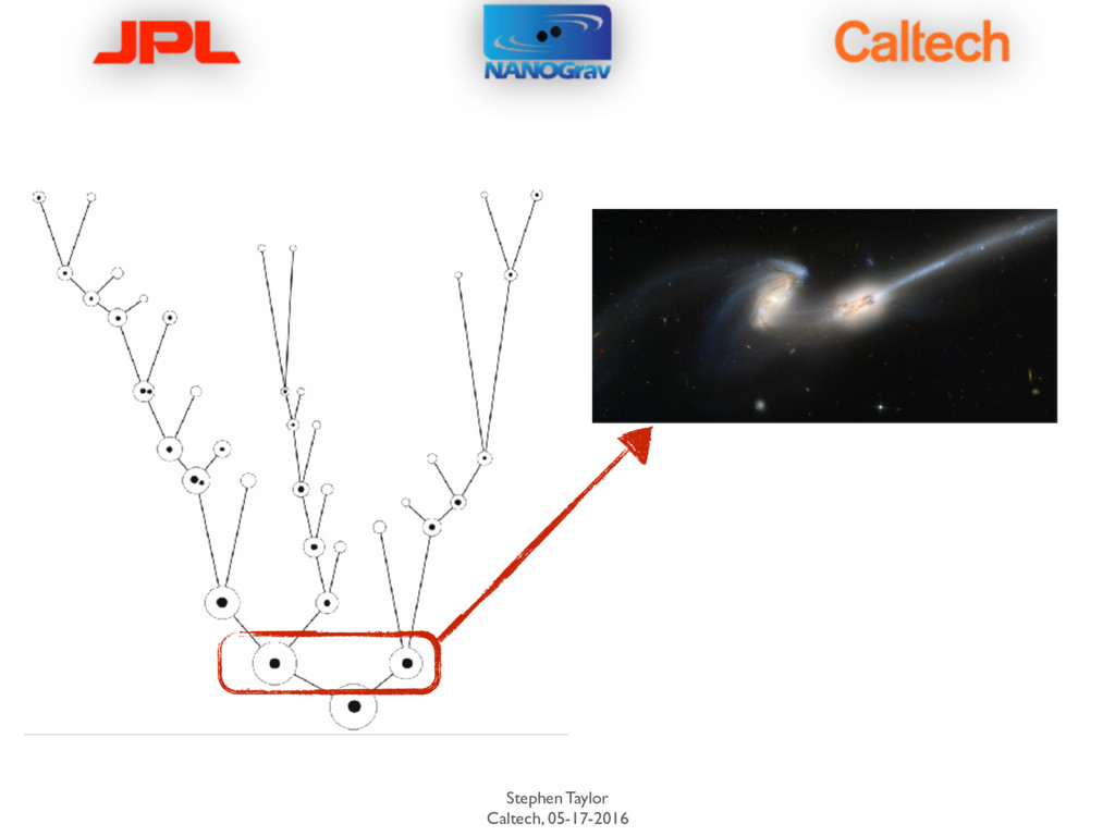
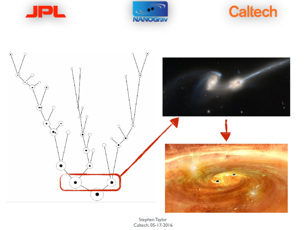
thought to form ubiquitously within models of galaxy formation Supermassive black holes are copious in the nuclei of nearby galaxies Several relationships exhibit coevolution between galactic bulge properties and the central black hole Current paradigm of galaxy formation is that galaxies undergo repeated merger events, and accrete from cosmic web filaments (White & Rees, 1978) DeLucia & Blaizot (2007) Quick detour: Sources
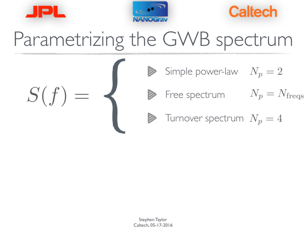
signal from these binaries? Phinney (2001) hc(f)2 / X i h2 i f C i r c u l a r, G W - d r i v e n population Quick detour: Sources Characteristic strain-spectrum — PSD of timing residuals — S(f) = hc(f)2 12⇡2 = A2 gwb 12⇡2 ✓ f yr 1 ◆ 13/3 yr3 hc(f) = Agwb ✓ f yr 1 ◆ 2/3 Time-domain covariance of residuals — C ( ti, tj)gwb = Z f high f low d f S ( f ) cos(2 ⇡f|ti tj | ) f3
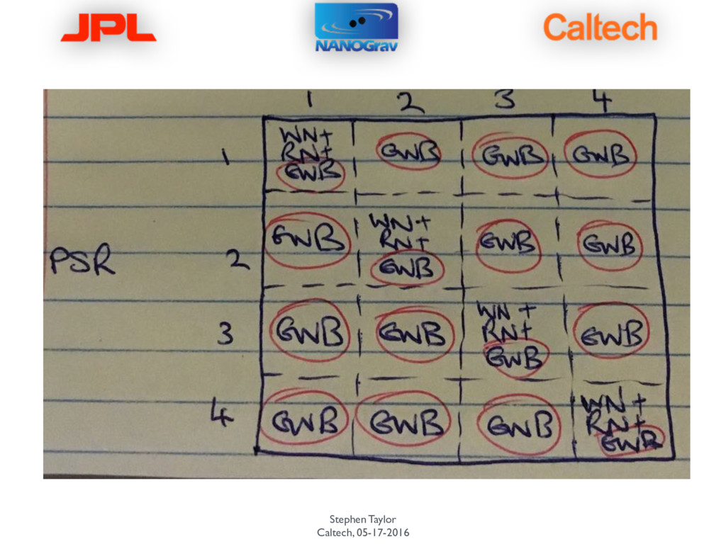
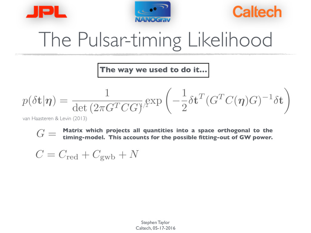
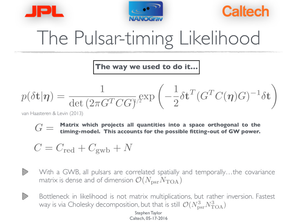
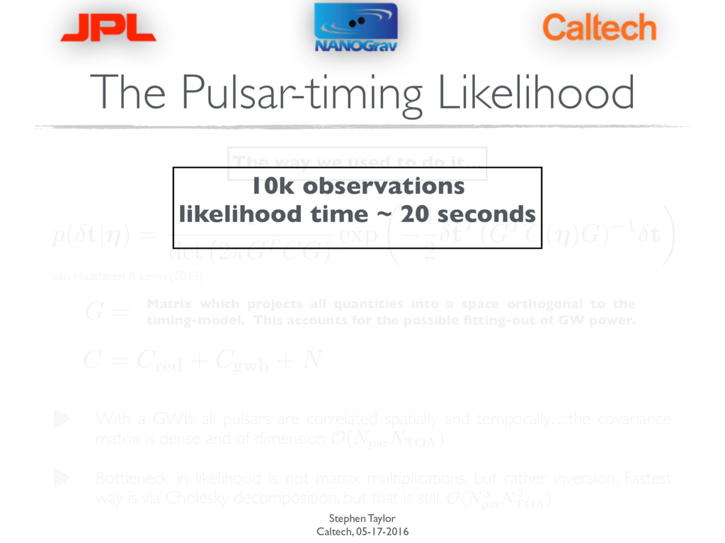
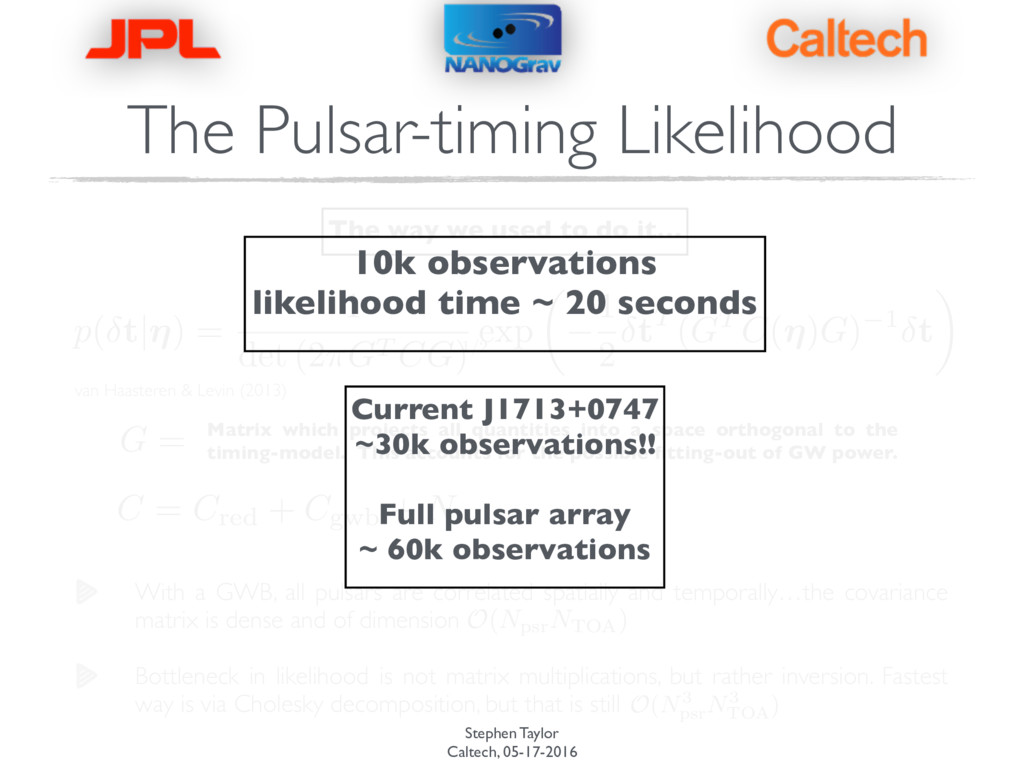
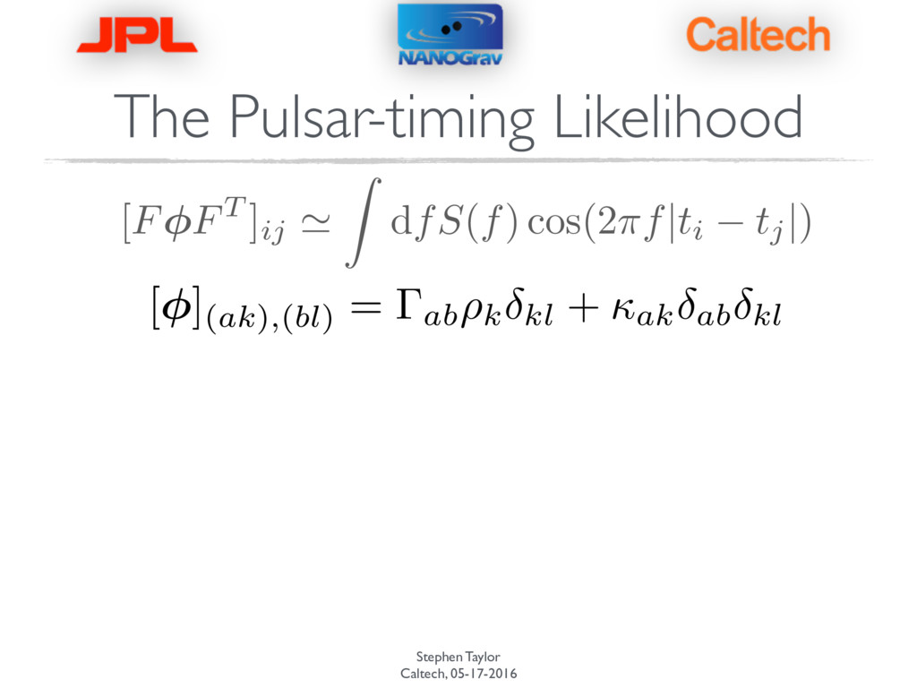
Pulsar-timing Likelihood p ( t|⌘ ) = 1 det (2 ⇡GT CG ) exp ✓ 1 2 tT ( GT C ( ⌘ ) G ) 1 t ◆ The way we used to do it… Matrix which projects all quantities into a space orthogonal to the timing-model. This accounts for the possible fitting-out of GW power. G = C = Cred + Cgwb + N 1/2
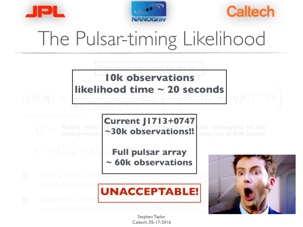
Pulsar-timing Likelihood p ( t|⌘ ) = 1 det (2 ⇡GT CG ) exp ✓ 1 2 tT ( GT C ( ⌘ ) G ) 1 t ◆ The way we used to do it… Matrix which projects all quantities into a space orthogonal to the timing-model. This accounts for the possible fitting-out of GW power. G = C = Cred + Cgwb + N 1/2 O(NpsrNTOA) With a GWB, all pulsars are correlated spatially and temporally…the covariance matrix is dense and of dimension Bottleneck in likelihood is not matrix multiplications, but rather inversion. Fastest way is via Cholesky decomposition, but that is still O(N3 psr N3 TOA )
Pulsar-timing Likelihood p ( t|⌘ ) = 1 det (2 ⇡GT CG ) exp ✓ 1 2 tT ( GT C ( ⌘ ) G ) 1 t ◆ The way we used to do it… Matrix which projects all quantities into a space orthogonal to the timing-model. This accounts for the possible fitting-out of GW power. G = C = Cred + Cgwb + N 1/2 O(NpsrNTOA) With a GWB, all pulsars are correlated spatially and temporally…the covariance matrix is dense and of dimension Bottleneck in likelihood is not matrix multiplications, but rather inversion. Fastest way is via Cholesky decomposition, but that is still O(N3 psr N3 TOA ) 10k observations likelihood time ~ 20 seconds
Pulsar-timing Likelihood p ( t|⌘ ) = 1 det (2 ⇡GT CG ) exp ✓ 1 2 tT ( GT C ( ⌘ ) G ) 1 t ◆ The way we used to do it… Matrix which projects all quantities into a space orthogonal to the timing-model. This accounts for the possible fitting-out of GW power. G = C = Cred + Cgwb + N 1/2 O(NpsrNTOA) With a GWB, all pulsars are correlated spatially and temporally…the covariance matrix is dense and of dimension Bottleneck in likelihood is not matrix multiplications, but rather inversion. Fastest way is via Cholesky decomposition, but that is still O(N3 psr N3 TOA ) 10k observations likelihood time ~ 20 seconds Current J1713+0747 ~30k observations!! Full pulsar array ~ 60k observations
Pulsar-timing Likelihood p ( t|⌘ ) = 1 det (2 ⇡GT CG ) exp ✓ 1 2 tT ( GT C ( ⌘ ) G ) 1 t ◆ The way we used to do it… Matrix which projects all quantities into a space orthogonal to the timing-model. This accounts for the possible fitting-out of GW power. G = C = Cred + Cgwb + N 1/2 O(NpsrNTOA) With a GWB, all pulsars are correlated spatially and temporally…the covariance matrix is dense and of dimension Bottleneck in likelihood is not matrix multiplications, but rather inversion. Fastest way is via Cholesky decomposition, but that is still O(N3 psr N3 TOA ) 10k observations likelihood time ~ 20 seconds Current J1713+0747 ~30k observations!! Full pulsar array ~ 60k observations UNACCEPTABLE!
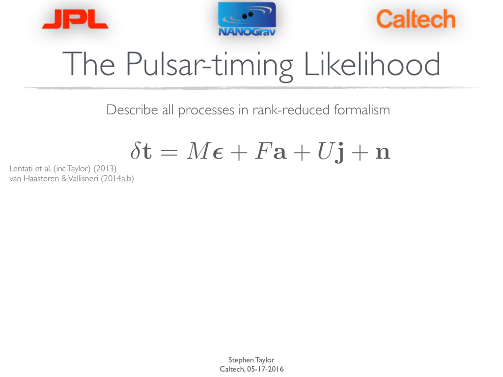
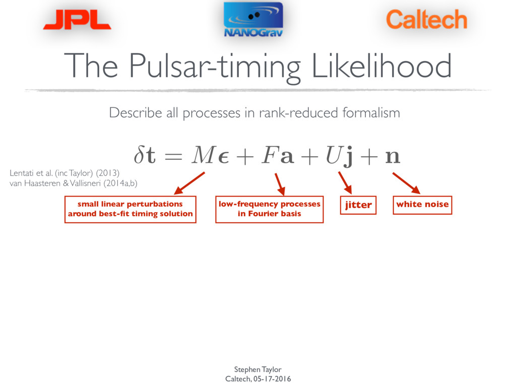
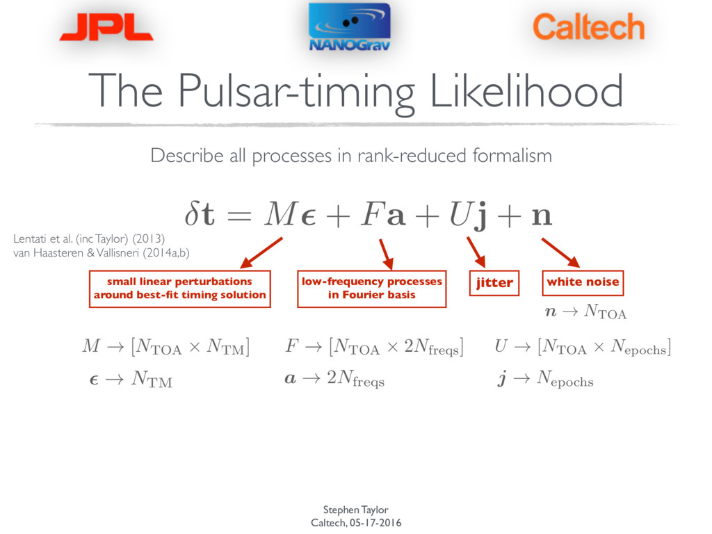
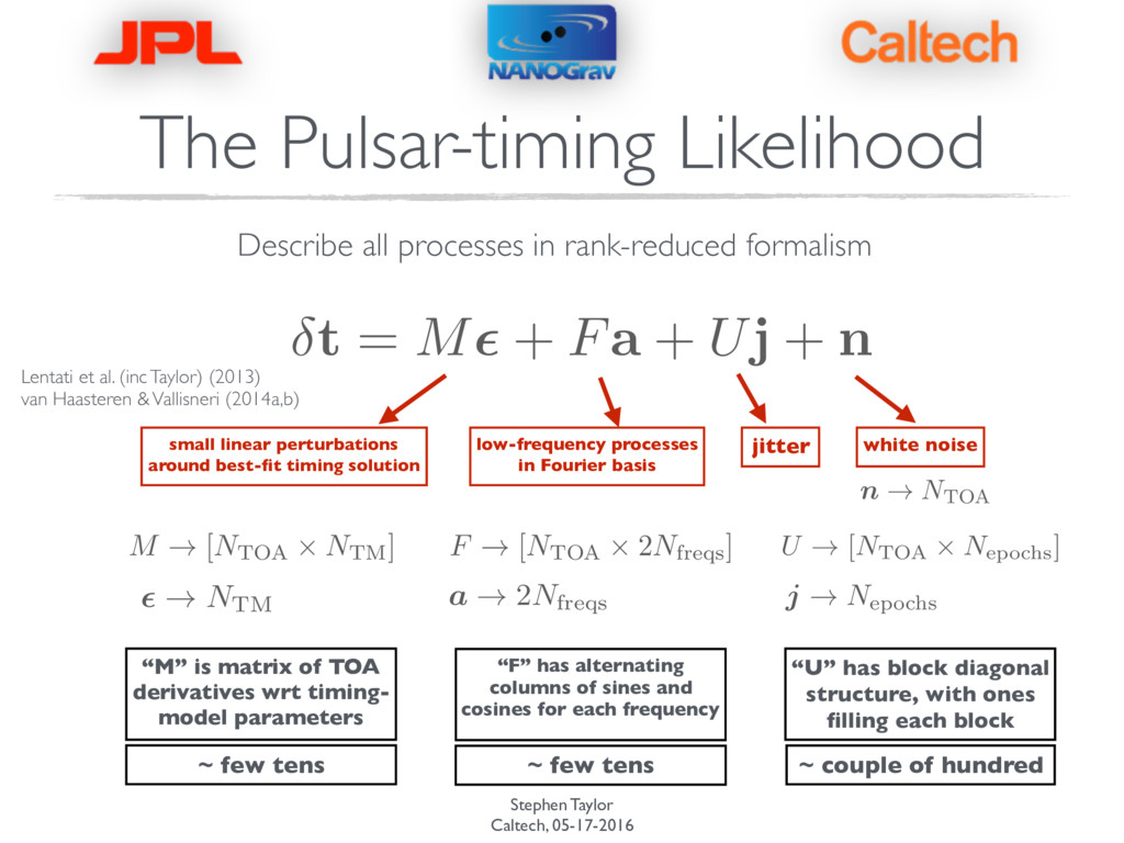
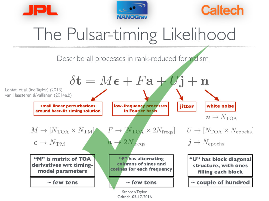
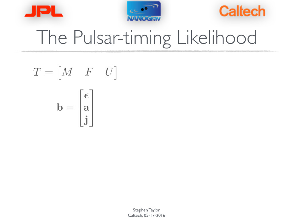
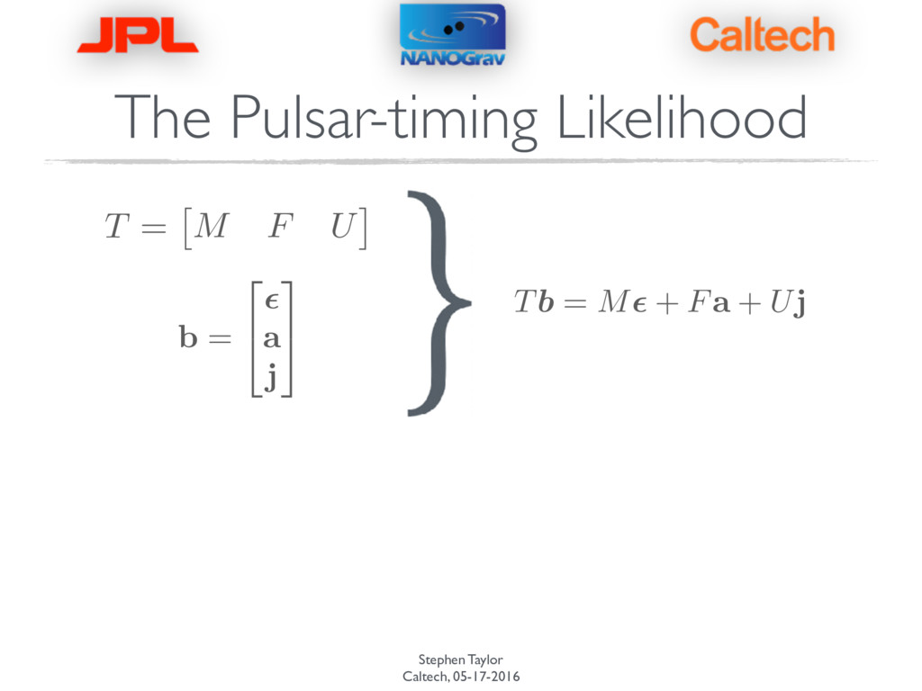
Uj + n The Pulsar-timing Likelihood Describe all processes in rank-reduced formalism Lentati et al. (inc Taylor) (2013) van Haasteren & Vallisneri (2014a,b)
Uj + n The Pulsar-timing Likelihood Describe all processes in rank-reduced formalism small linear perturbations around best-fit timing solution low-frequency processes in Fourier basis jitter white noise Lentati et al. (inc Taylor) (2013) van Haasteren & Vallisneri (2014a,b)
Uj + n The Pulsar-timing Likelihood Describe all processes in rank-reduced formalism small linear perturbations around best-fit timing solution low-frequency processes in Fourier basis jitter white noise M ! [NTOA ⇥ NTM] ✏ ! NTM F ! [NTOA ⇥ 2Nfreqs] a ! 2Nfreqs U ! [NTOA ⇥ Nepochs] j ! N epochs n ! NTOA Lentati et al. (inc Taylor) (2013) van Haasteren & Vallisneri (2014a,b)
Uj + n The Pulsar-timing Likelihood Describe all processes in rank-reduced formalism small linear perturbations around best-fit timing solution low-frequency processes in Fourier basis jitter white noise M ! [NTOA ⇥ NTM] ✏ ! NTM F ! [NTOA ⇥ 2Nfreqs] a ! 2Nfreqs U ! [NTOA ⇥ Nepochs] j ! N epochs n ! NTOA ~ few tens ~ few tens ~ couple of hundred “M” is matrix of TOA derivatives wrt timing- model parameters “F” has alternating columns of sines and cosines for each frequency “U” has block diagonal structure, with ones filling each block Lentati et al. (inc Taylor) (2013) van Haasteren & Vallisneri (2014a,b)
Uj + n The Pulsar-timing Likelihood Describe all processes in rank-reduced formalism small linear perturbations around best-fit timing solution low-frequency processes in Fourier basis jitter white noise M ! [NTOA ⇥ NTM] ✏ ! NTM F ! [NTOA ⇥ 2Nfreqs] a ! 2Nfreqs U ! [NTOA ⇥ Nepochs] j ! N epochs n ! NTOA ~ few tens ~ few tens ~ couple of hundred “M” is matrix of TOA derivatives wrt timing- model parameters “F” has alternating columns of sines and cosines for each frequency “U” has block diagonal structure, with ones filling each block Lentati et al. (inc Taylor) (2013) van Haasteren & Vallisneri (2014a,b)
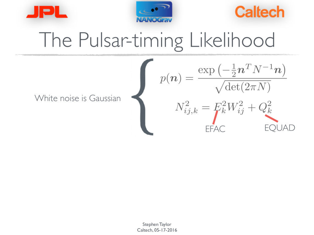
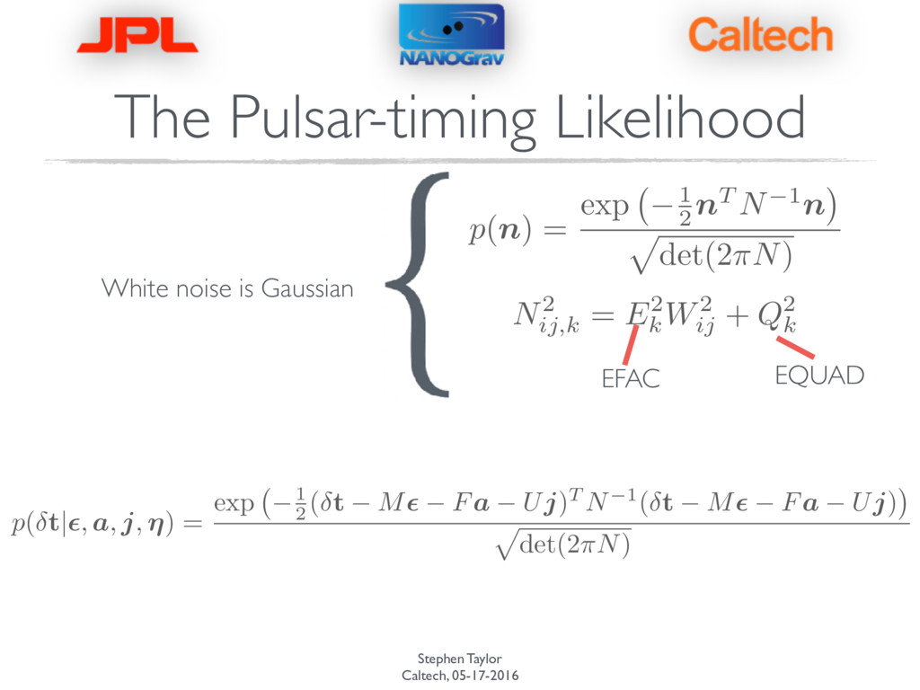
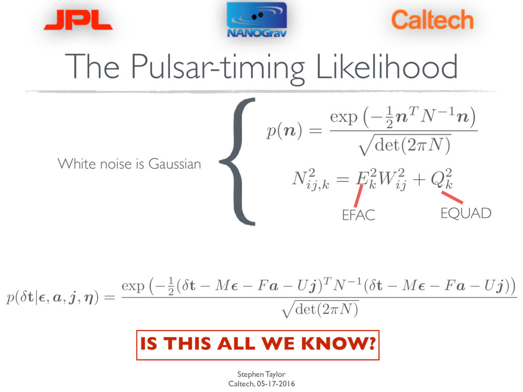
) = exp 1 2 nT N 1n p det(2 ⇡N ) White noise is Gaussian N2 ij,k = E2 k W2 ij + Q2 k EFAC EQUAD p ( t|✏, a, j, ⌘ ) = exp 1 2 ( t M✏ Fa Uj ) T N 1 ( t M✏ Fa Uj ) p det(2 ⇡N )
) = exp 1 2 nT N 1n p det(2 ⇡N ) White noise is Gaussian N2 ij,k = E2 k W2 ij + Q2 k EFAC EQUAD p ( t|✏, a, j, ⌘ ) = exp 1 2 ( t M✏ Fa Uj ) T N 1 ( t M✏ Fa Uj ) p det(2 ⇡N ) IS THIS ALL WE KNOW?
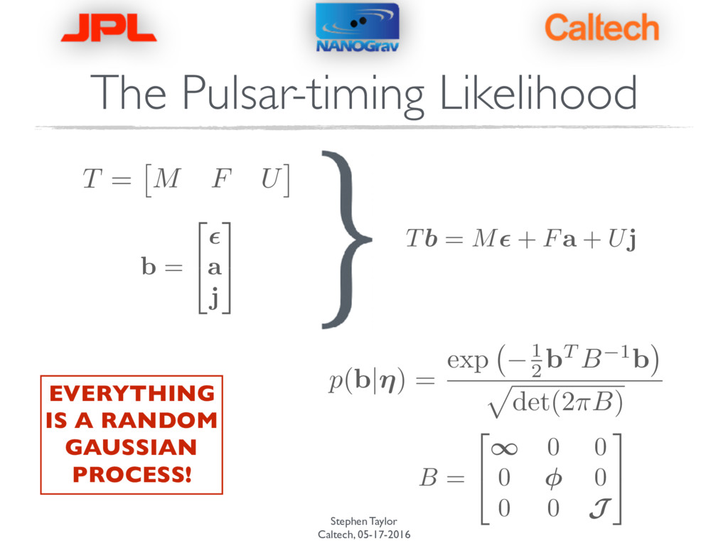
M F U ⇤ b = 2 4 ✏ a j 3 5 Tb = M✏ + Fa + Uj EVERYTHING IS A RANDOM GAUSSIAN PROCESS! p ( b|⌘ ) = exp 1 2 bT B 1b p det(2 ⇡B ) B = 2 4 1 0 0 0 0 0 0 J 3 5
M F U ⇤ b = 2 4 ✏ a j 3 5 Tb = M✏ + Fa + Uj EVERYTHING IS A RANDOM GAUSSIAN PROCESS! p ( b|⌘ ) = exp 1 2 bT B 1b p det(2 ⇡B ) B = 2 4 1 0 0 0 0 0 0 J 3 5
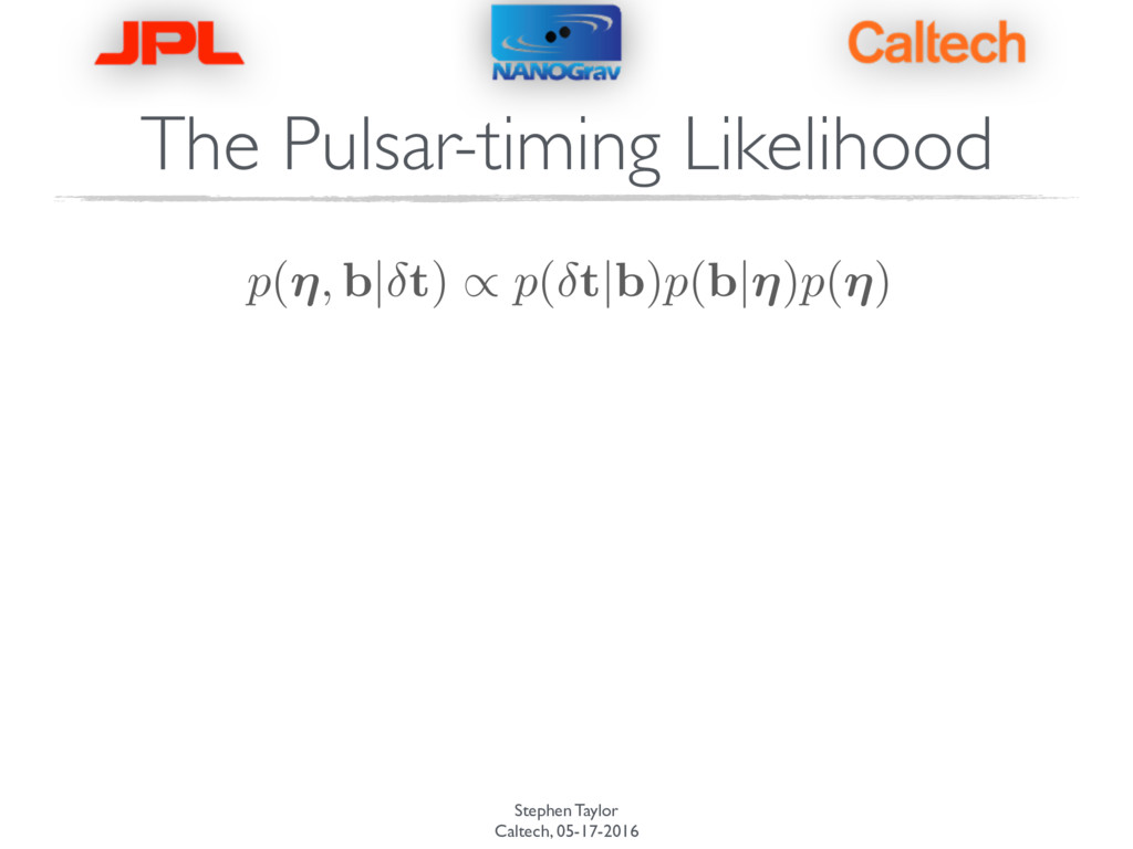
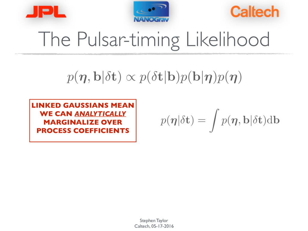
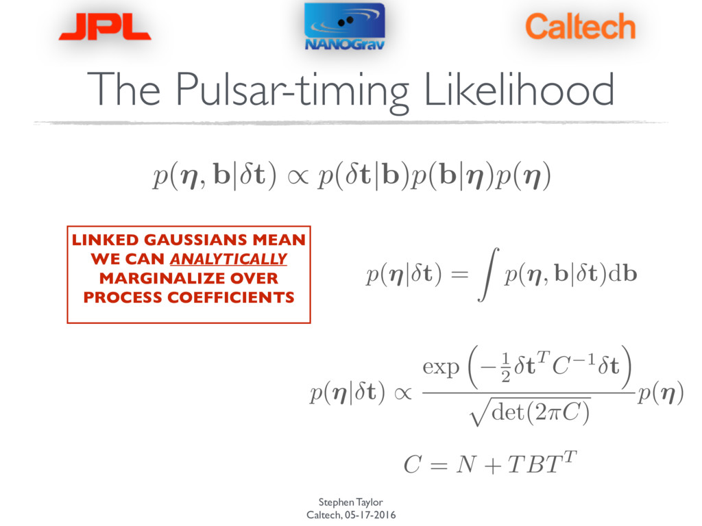
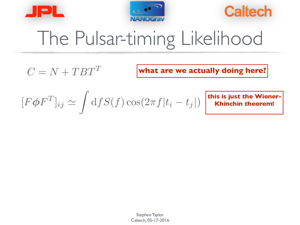
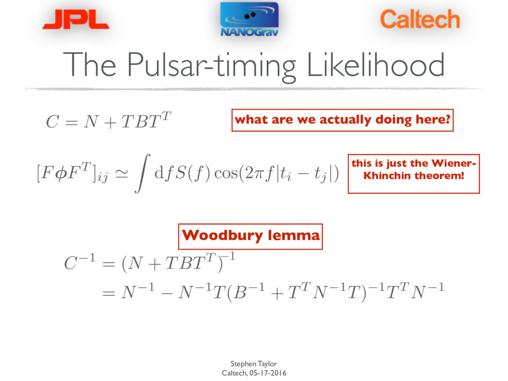
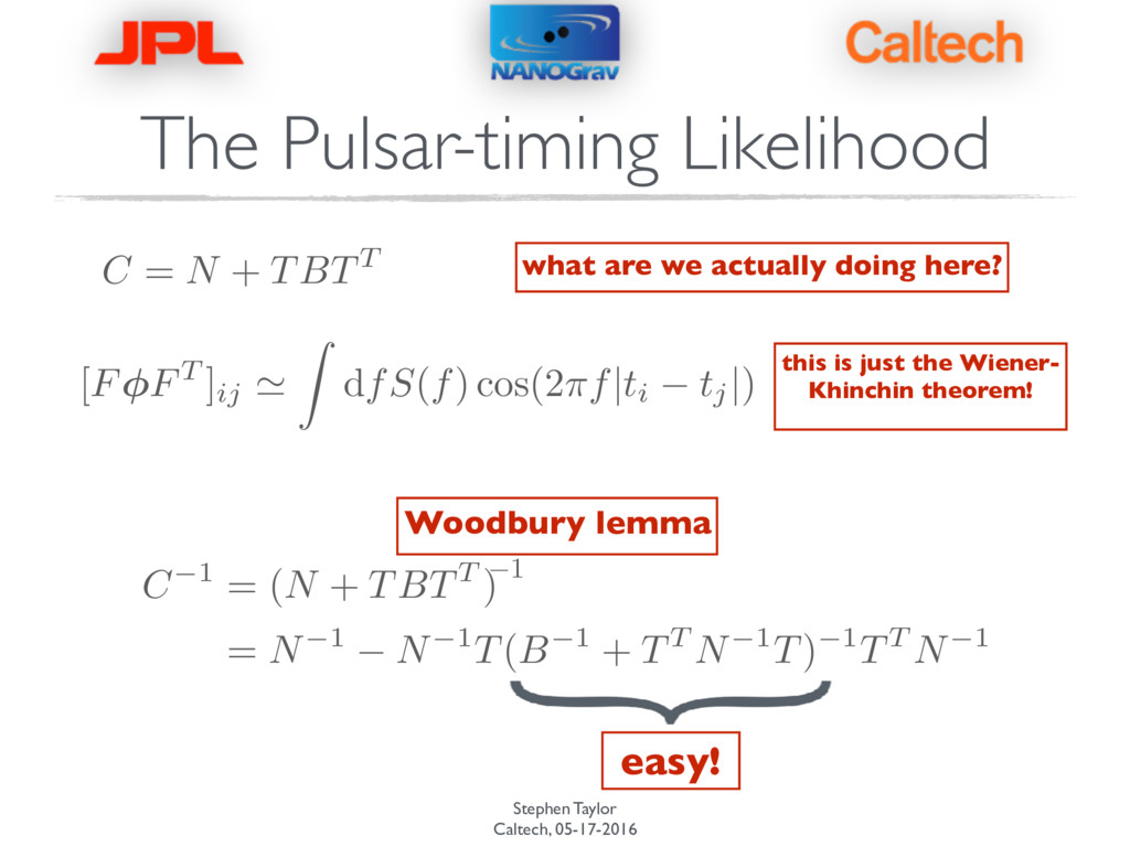
WE CAN ANALYTICALLY MARGINALIZE OVER PROCESS COEFFICIENTS p(⌘| t) = Z p(⌘, b| t)db p(⌘, b| t) / p( t|b)p(b|⌘)p(⌘) p ( ⌘| t ) / exp ⇣ 1 2 tT C 1 t ⌘ p det(2 ⇡C ) p ( ⌘ ) C = N + TBTT
WE CAN ANALYTICALLY MARGINALIZE OVER PROCESS COEFFICIENTS p(⌘| t) = Z p(⌘, b| t)db p(⌘, b| t) / p( t|b)p(b|⌘)p(⌘) p ( ⌘| t ) / exp ⇣ 1 2 tT C 1 t ⌘ p det(2 ⇡C ) p ( ⌘ ) C = N + TBTT
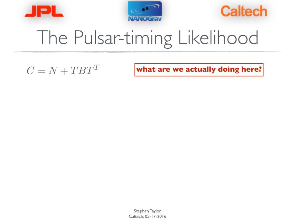
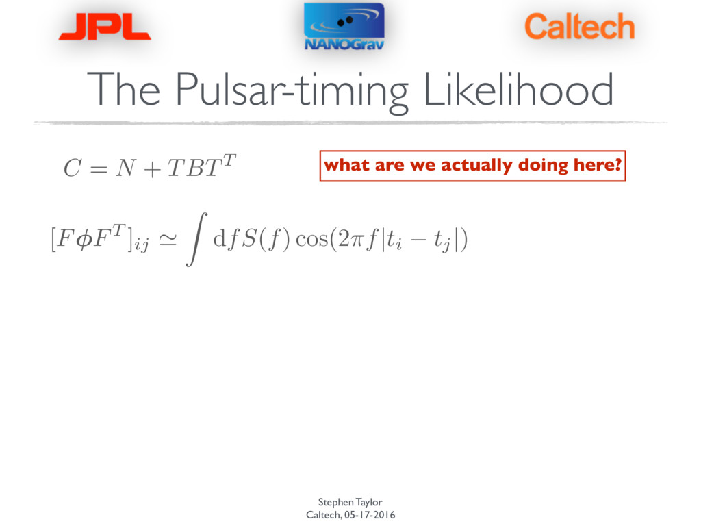
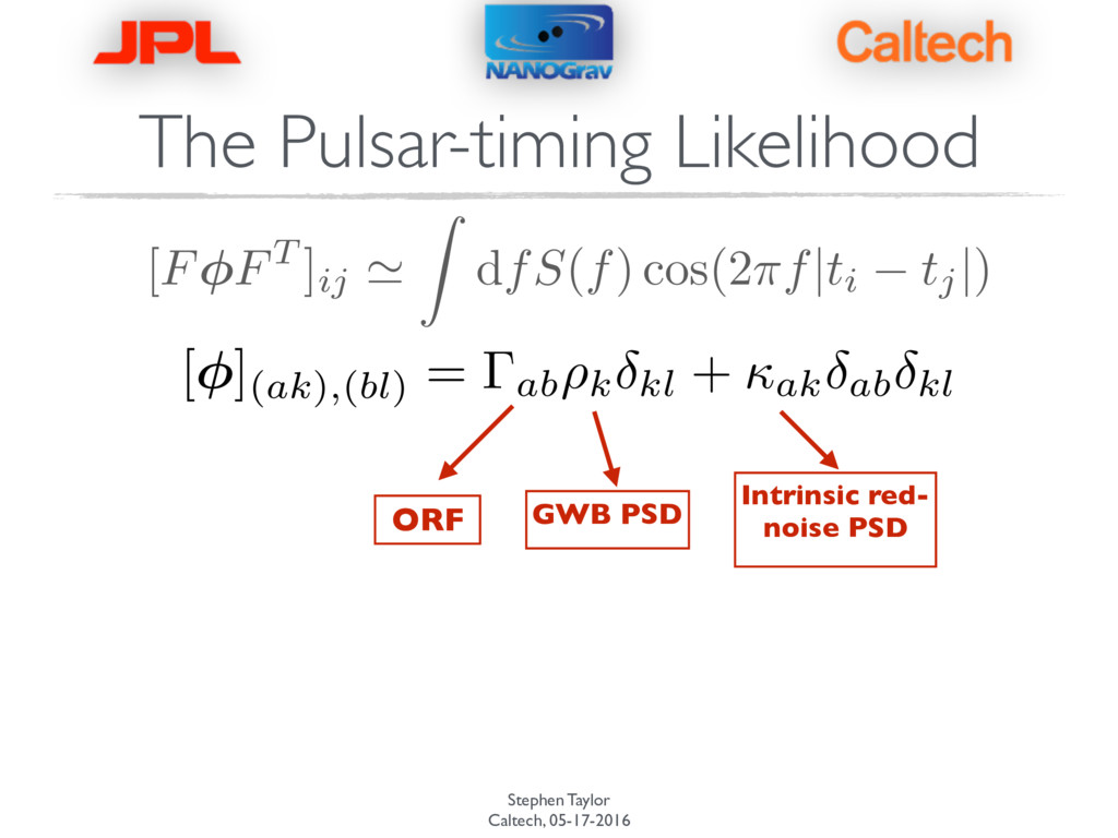
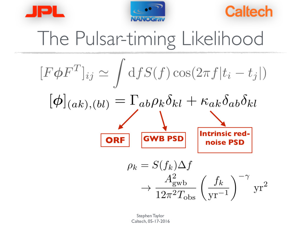
+ TBTT what are we actually doing here? this is just the Wiener- Khinchin theorem! [ F FT ]ij ' Z d fS ( f ) cos(2 ⇡f|ti tj | ) C 1 = (N + TBTT ) = N 1 N 1T(B 1 + TT N 1T) 1TT N 1 Woodbury lemma 1
+ TBTT what are we actually doing here? this is just the Wiener- Khinchin theorem! [ F FT ]ij ' Z d fS ( f ) cos(2 ⇡f|ti tj | ) C 1 = (N + TBTT ) = N 1 N 1T(B 1 + TT N 1T) 1TT N 1 easy! Woodbury lemma 1
Intrinsic red- noise PSD [ F FT ]ij ' Z d fS ( f ) cos(2 ⇡f|ti tj | ) [ ](ak),(bl) = ab⇢k kl + ak ab kl ⇢k = S(fk) f ! A2 gwb 12⇡2 T obs ✓ fk yr 1 ◆ yr2
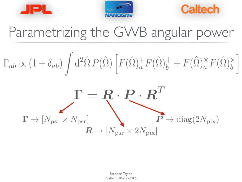
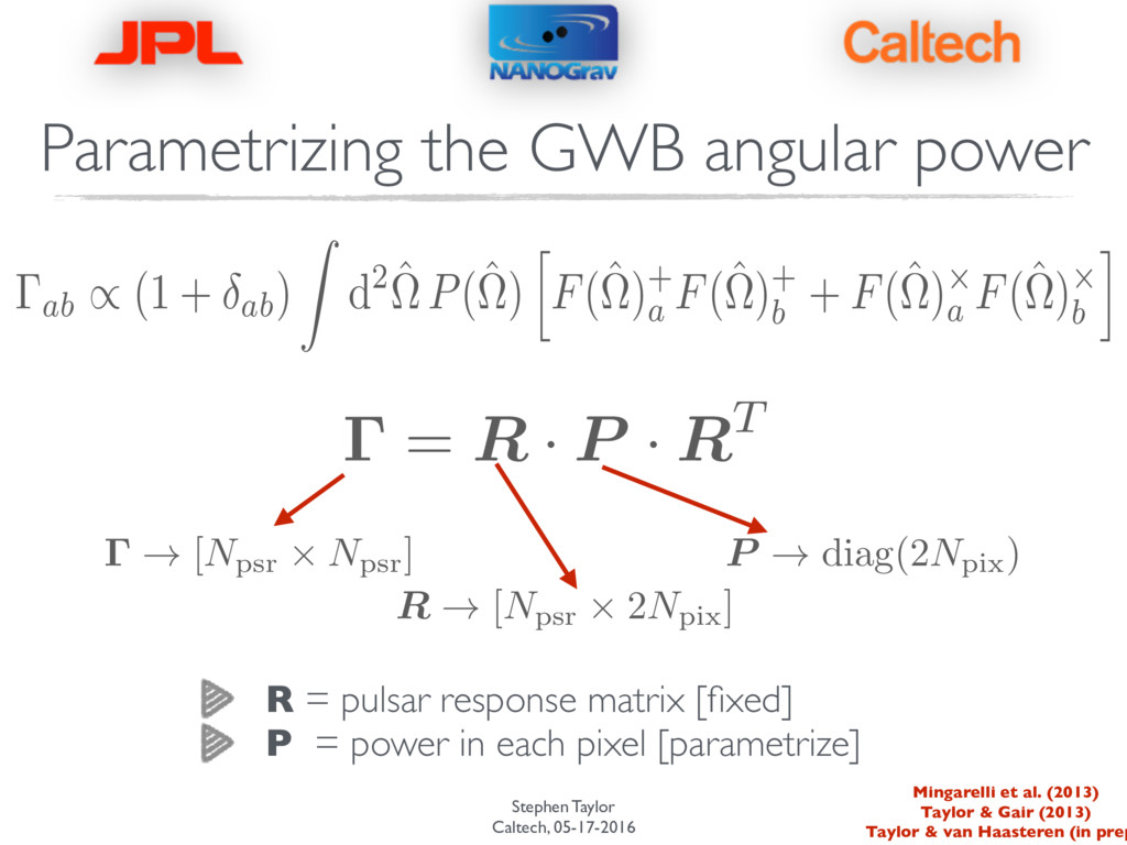
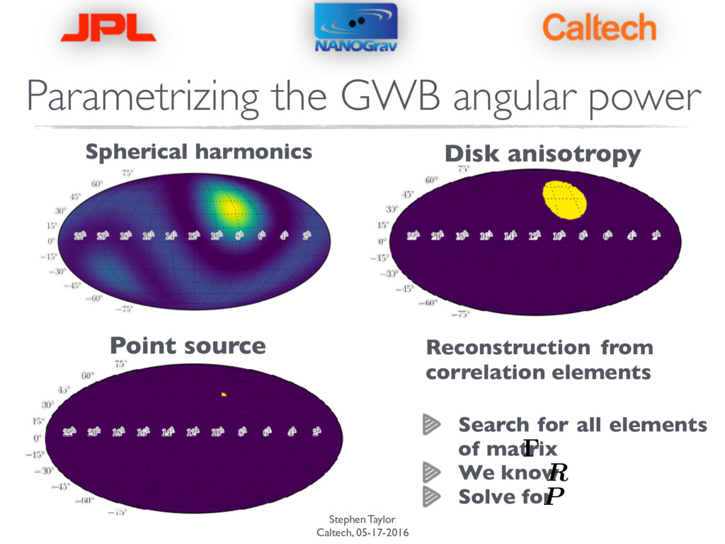
/ (1 + ab) Z d2 ˆ ⌦P(ˆ ⌦) h F(ˆ ⌦)+ a F(ˆ ⌦)+ b + F(ˆ ⌦)⇥ a F(ˆ ⌦)⇥ b i = R · P · RT R ! [N psr ⇥ 2N pix ] P ! diag(2N pix ) ! [Npsr ⇥ Npsr] R = pulsar response matrix [fixed] P = power in each pixel [parametrize] Mingarelli et al. (2013) Taylor & Gair (2013) Taylor & van Haasteren (in prep
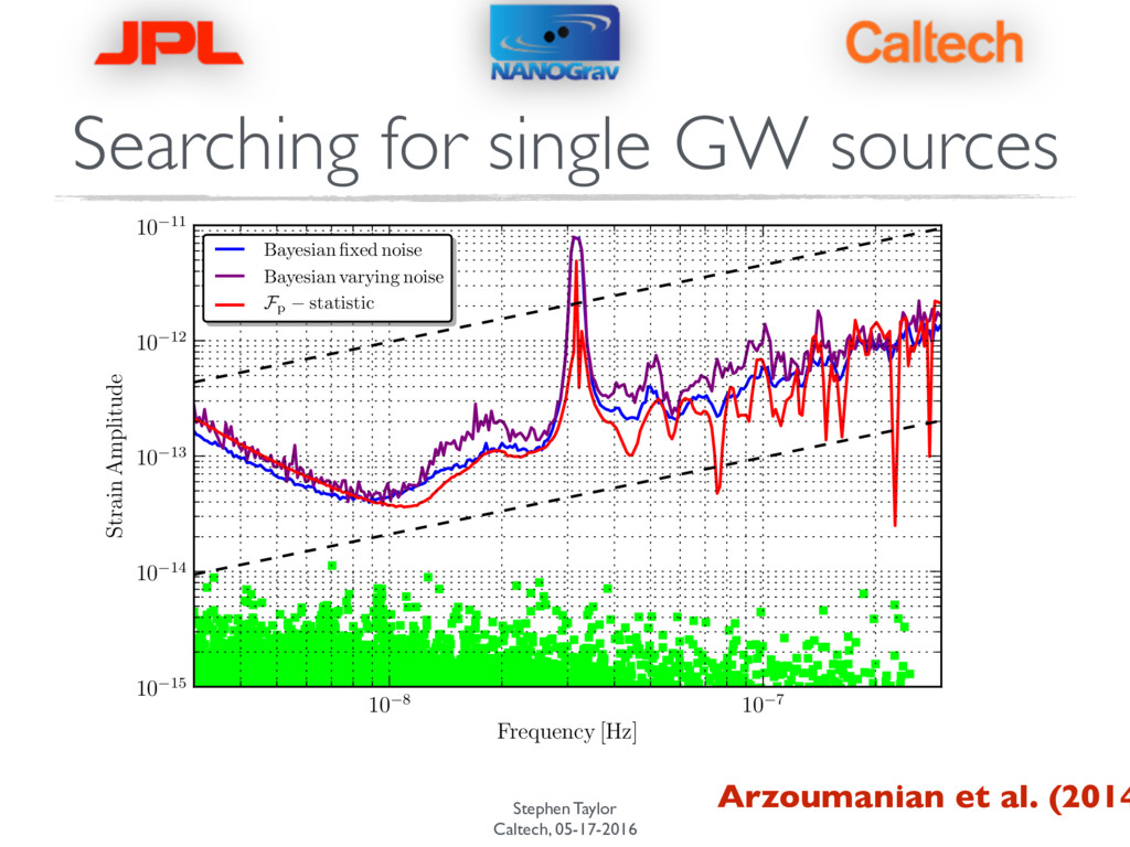
[Hz] 10 15 10 14 10 13 10 12 10 11 Strain Amplitude Bayesian fixed noise Bayesian varying noise Fp statistic Figure 5. Sky-averaged upper limit on the strain amplitude, h 0 as a function of GW frequency. The Bayesian upper limits are computed using a fixed-noise model (thick black(blue)) and a varying noise model (thin black(purple)) and the frequentist upper limit (gray(red)) is computed using the Fp-statistic. The dashed curves indicate lines of constant chirp mass for a source with a distance to the Virgo cluster (16.5 Mpc) and chirp mass of 109M (lower) and 1010M (upper). The gray(green) squares show the strain amplitude of the loudest GW sources in 1000 monte-carlo realizations using an optimistic phenomenological Arzoumanian et al. (2014 Searching for single GW sources
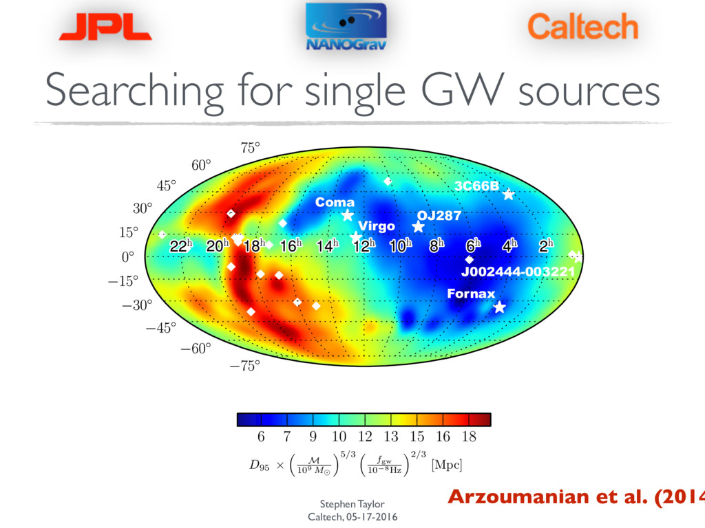
⌘5/3 ⇣ fgw 10 8Hz ⌘2/3 [Mpc] Figure 6. 95% lower limit on the luminosity distance as a function of sky location computed using the Fp-statistic plotted in equatorial coordinates . The values in the colorbar are calculated assuming a chirp mass of M = 109M and a GW frequency f gw = 1 ⇥ 10-8 Hz. The white diamonds denote the locations of the pulsars in the sky and the black(white) stars denote possible SMBHBs or clusters possibly containing SMBHBs. As expected from the antenna pattern functions of the pulsars, we are most sensitive to GWs from sky locations near the pulsars. The luminosity distances to the potential sources are 92.3, 1575.5, 2161.7, 16.5, 104.5, and 19 Mpc for 3C66B, OJ287, J002444-003221, Virgo Cluster, Coma Cluster, and Fornax Cluster, respectively. (Color figure available in the online version.) 6 7 9 10 12 13 15 16 18 D95 ⇥ ⇣ M 109 M ⌘5/3 ⇣ fgw 10 8Hz ⌘2/3 [Mpc] Coma Virgo OJ287 Fornax 3C66B J002444-003221 Figure 7. 95% lower limit on the luminosity distance as a function of sky location computed using the Bayesian method including the noise model. The values in the colorbar are calculated assuming a chirp mass of M = 109M and a GW frequency f gw = 1 ⇥ 10-8 Hz. The white diamonds denote the locations of the Arzoumanian et al. (2014 Searching for single GW sources
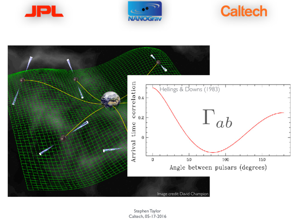
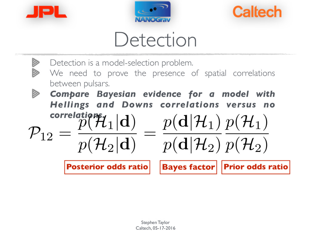
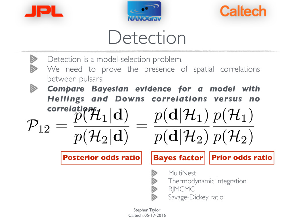
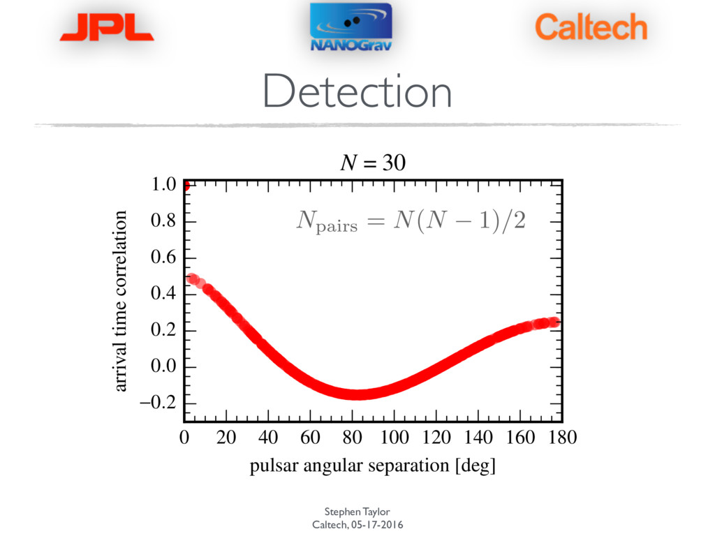
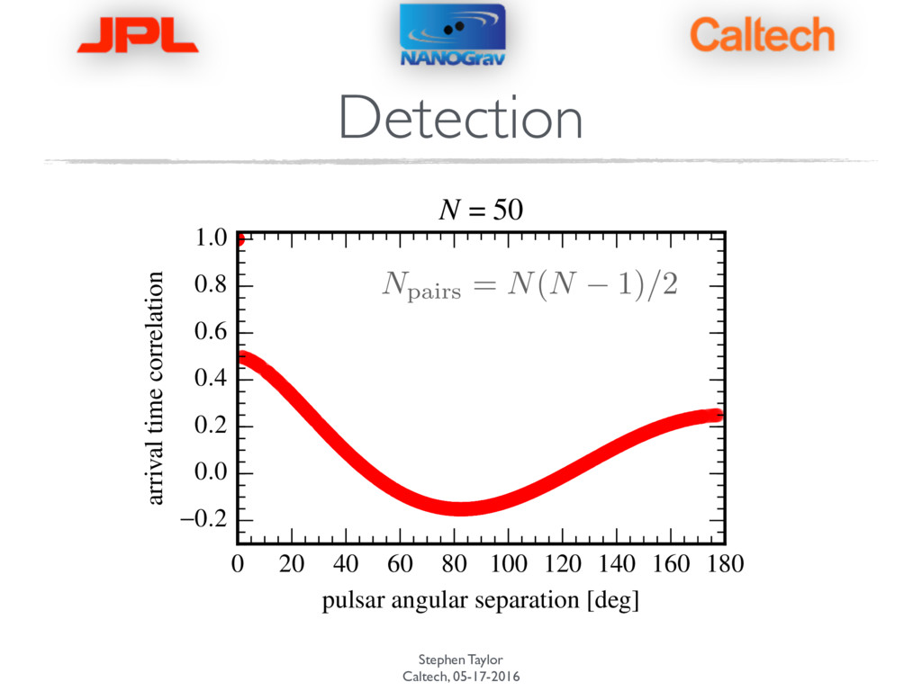
We need to prove the presence of spatial correlations between pulsars. Compare Bayesian evidence for a model with Hellings and Downs correlations versus no correlations.
We need to prove the presence of spatial correlations between pulsars. Compare Bayesian evidence for a model with Hellings and Downs correlations versus no correlations. P12 = p(H1 |d) p(H2 |d) = p(d|H1) p(d|H2) p(H1) p(H2) Posterior odds ratio Bayes factor Prior odds ratio
We need to prove the presence of spatial correlations between pulsars. Compare Bayesian evidence for a model with Hellings and Downs correlations versus no correlations. P12 = p(H1 |d) p(H2 |d) = p(d|H1) p(d|H2) p(H1) p(H2) Posterior odds ratio Bayes factor Prior odds ratio MultiNest Thermodynamic integration RJMCMC Savage-Dickey ratio
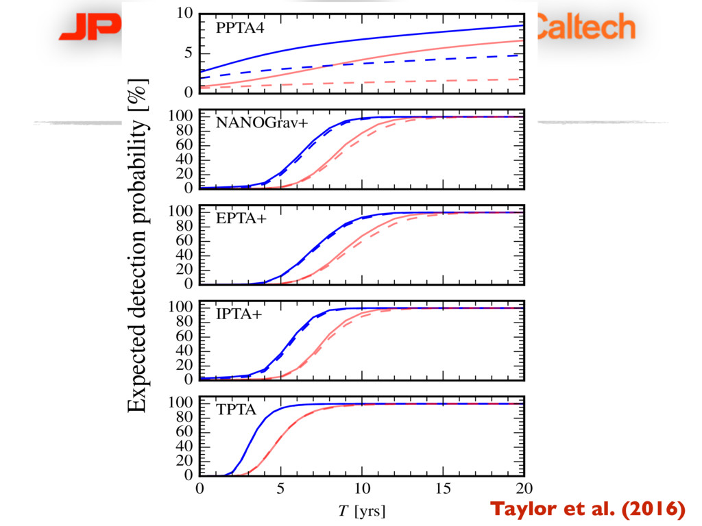
problem We use hierarchical Bayesian modeling and sophisticated MCMC techniques to search for correlations between tens of pulsars We will soon need a new paradigm to permit ~100 pulsars to be used in the searches Detection within 10 years pretty favorable Lots of interesting astrophysics to probe
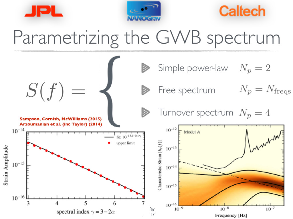
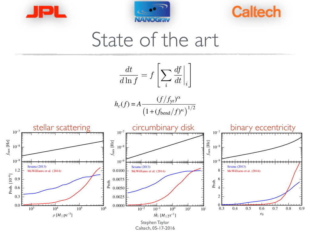
in dataset does some- data set results in the prior distribu- inform the prior at d update the prior. mits nvironmental cou- WB signal at low ) via a simple pa- allows for a “bend” m environmentally- The following dis- the dt/d ln f term) of this equation (see Colpi 2014, for a review of SMBHB coalescence). Following Sampson et al. (2015) we can generalize the frequency dependence of the strain spectrum to dt d ln f = f ✓ d f dt ◆-1 = f X i ✓ d f dt ◆ i !-1 , (23) where i ranges over many physical processes that are driv- ing the binary to coalescence. If we restrict this sum to GW- driven evolution and an unspecified physical process then the strain spectrum is now hc (f) = A (f/fyr )↵ 1+(fbend/f) 1/2 , (24) dt d ln f = f " X i df dt i # 16 10-9 10-8 10-7 fturn [Hz] 103 104 105 106 ⇢ [M pc-3] 0.0 0.3 0.6 0.9 1.2 Prob. [10-6] Sesana (2013) McWilliams et al. (2014) Figure 10. (top): Empirical mapping from fturn to ⇢ (left) and ˙ M1 (right). (bottom): Posterior distributions for the mass density of stars in the galactic core 10-9 10-8 10-7 fturn [Hz] 10-2 10-1 100 101 102 ˙ M1 [M yr-1] 0.0000 0.0025 0.0050 0.0075 0.0100 Prob. Sesana (2013) McWilliams et al. (2014) 10. (top): Empirical mapping from fturn to ⇢ (left) and ˙ M1 (right). (bottom): Posterior distributions for the mass density of stars in the galactic core 16 Figure 10. (top): Empirical mapping from fturn to ⇢ (left) and ˙ M1 (right). (bottom): Posterior distributions for the mass density of stars in the galactic core (left) and the accretion rate of the primary black hole from a circumbinary disk (right). These distributions are constructed by first converting the marginalized distribution of fbend to a distribution of fturn via Eq. (30), and then using the empirical mapping described in the text to convert from fturn to the astrophysical quantities ⇢ and ˙ M1, respectively. raise the stellar mass density to match a corresponding in- crease in binary mass so that the transition frequency is main- tained. Furthermore, modeling the distribution of black holes masses in Eq. (35) without the lognormal component or red- shift evolution will increase the contribution of lower mass binaries to the GW strain budget, leading to smaller stellar mass density constraints than reported in Fig. 10. Varying the normalization, a, and exponent, b, of the M - relation such that a 2 [7,9] and b 2 [4,6] has very little impact on the envi- ronmental constraints. 5.1.3. Constraints on SMBH binary population eccentricity It is not only the astrophysical environment of SMBH bi- naries that can induce a bend in the characteristic strain spec- trum. Binaries with non-zero eccentricity emit GWs at a spec- trum of harmonics of the orbital frequency. The cumulative effect over the entire population can lead to a depletion of the low frequency strain spectrum (Enoki et al. 2007; Sesana 2013; Ravi et al. 2014; Huerta et al. 2015), and a turnover whose shape can be captured with the parametrized spectrum model employed in this paper. Hence, we can use our fturn posterior from the marginalization of fbend over all to de- duce constraints on the eccentricity of binaries at some refer- 10-9 10-8 10-7 fturn [Hz] 0.3 0.4 0.5 0.6 0.7 0.8 0.9 e0 0 2 4 6 8 Prob. Sesana (2013) McWilliams et al. (2014) Figure 11. Same as Figure 10 except now we display the empirical map- ping (top) and posterior distribution (bottom) for the eccentricity of SMBH stellar scattering circumbinary disk binary eccentricity
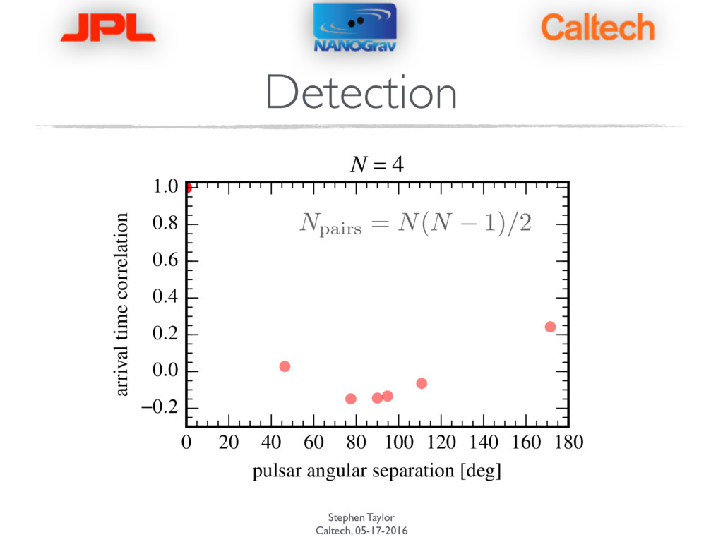
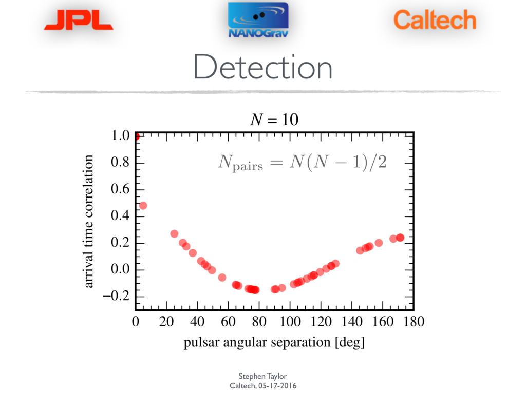
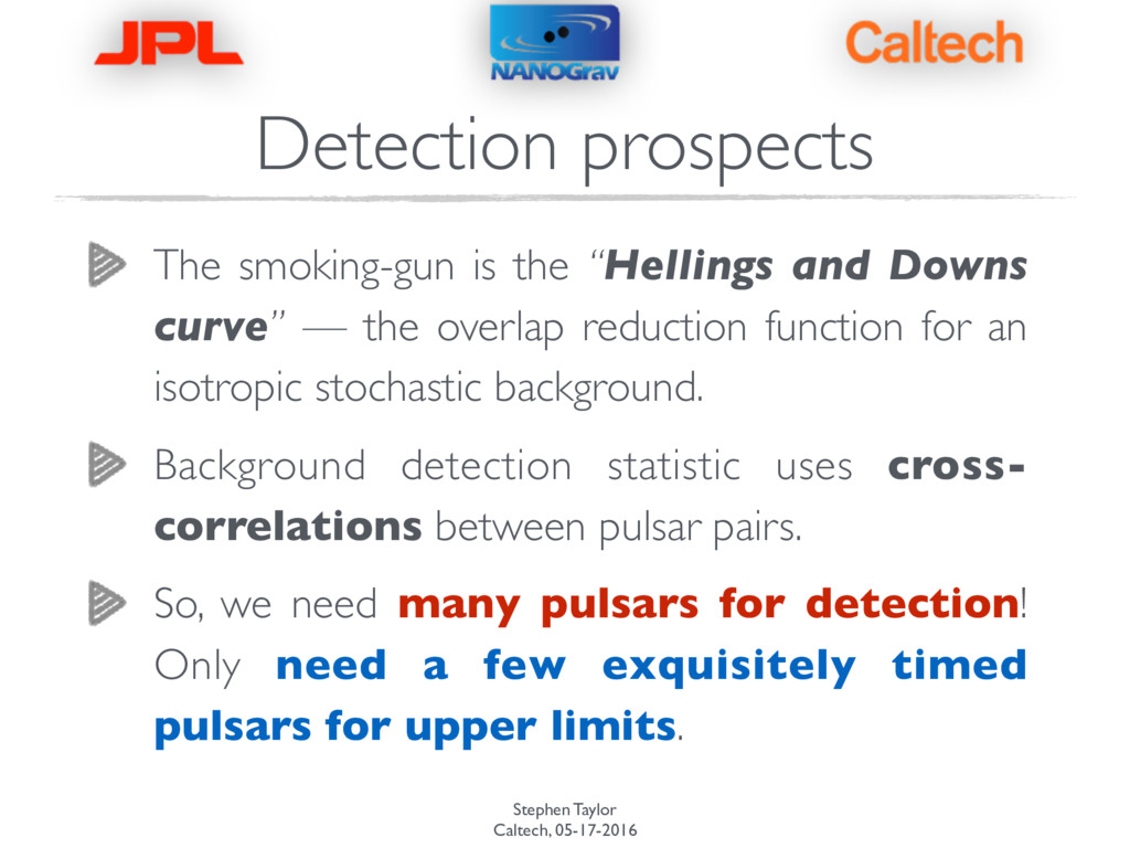
Downs curve” — the overlap reduction function for an isotropic stochastic background. Background detection statistic uses cross- correlations between pulsar pairs. So, we need many pulsars for detection! Only need a few exquisitely timed pulsars for upper limits. Detection prospects