Risk Estimation for the Group Lasso

SPARS'13, EPFL, Lausanne, August 2013

Transcript

1. Risk Estimation for the Group Lasso (and its degrees of freedom) Samuel VAITER CNRS, Université Paris-Dauphine, France Joint work with C. DELEDALLE, G. PEYRÉ, J. FADILI and C. DOSSAL
2. Meet Lena inpainting denoising super-resolution
3. Linear Inverse Problems x0 RN unknown signal linear operator Y = x0 +W W white gaussian noise Y observations Forward model
4. Linear Inverse Problems x0 RN unknown signal linear operator Y = x0 +W W white gaussian noise Y observations Forward model y = x0 + w Realization
5. Linear Inverse Problems x0 RN unknown signal linear operator Objective Recover x0 from y Y = x0 +W W white gaussian noise Y observations Forward model y = x0 + w Realization
6. Linear Inverse Problems x0 RN unknown signal linear operator Objective Recover x0 from y How ? Construction of an estimator x(y) Y = x0 +W W white gaussian noise Y observations Forward model y = x0 + w Realization
7. Variational Regularization x (y) arg min x RN 1 2 y x 2 + J(x)
8. Variational Regularization x (y) arg min x RN 1 2 y x 2 + J(x) Fidelity Regularity
9. Variational Regularization x (y) arg min x RN 1 2 y x 2 + J(x) How ? Risk Estimation Objective Find such that x (y) x0 Fidelity Regularity
10. Variational Regularization x (y) arg min x RN 1 2 y x 2 + J(x) How ? Risk Estimation Objective Find such that x (y) x0 Fidelity Regularity Notations µ (y) = x (y) µ0 = x0
11. Risk Estimation projection risk AΦ = Φ∗(Φ∗Φ)+Φ = PKerΦ⊥ RA( ) = EW (Aµ0 Aµ (Y ))
12. Risk Estimation RId( ) projection risk AΦ = Φ∗(Φ∗Φ)+Φ = PKerΦ⊥ RA( ) = EW (Aµ0 Aµ (Y ))
13. Risk Estimation RId( ) Objective Minimize RA( ) over R+ projection risk AΦ = Φ∗(Φ∗Φ)+Φ = PKerΦ⊥ RA( ) = EW (Aµ0 Aµ (Y ))
14. (Generalized) Stein Unbiased Risk Estimation Sensitivity analysis: If µ weakly differentiable µ(y + ) = µ(y)+ µ(y)· +O( 2)
15. (Generalized) Stein Unbiased Risk Estimation Sensitivity analysis: If µ weakly differentiable µ(y + ) = µ(y)+ µ(y)· +O( 2) (Generalized) Stein Unbiased Risk Estimator GSUREA(y) = Ay Aµ(y) 2 2tr(A A)+2 2 ˆ dfA (y) ˆ dfA (y) = tr(A µ(y) A )
16. (Generalized) Stein Unbiased Risk Estimation Sensitivity analysis: If µ weakly differentiable µ(y + ) = µ(y)+ µ(y)· +O( 2) (Generalized) Stein Unbiased Risk Estimator GSUREA(y) = Ay Aµ(y) 2 2tr(A A)+2 2 ˆ dfA (y) ˆ dfA (y) = tr(A µ(y) A ) Lemma (Stein, ‘81 - Eldar, ‘09 - V. et al, ’12 ) EW (GSUREA(Y )) = EW (Aµ0 Aµ(Y ))
17. Lasso and Group Lasso supp(x) = {i : xi = 0} x 1 = |x1|+|x2|+|x3| x 1 = N i=1 |xi | [Dossal et al., 2012]
18. Lasso and Group Lasso supp(x) = {i : xi = 0} x 1 = |x1|+|x2|+|x3| x 1 = N i=1 |xi | x B = b∈B xb suppB (x) = {b : xb = 0} x B = x2 1 + x2 2 +|x3| [Dossal et al., 2012]
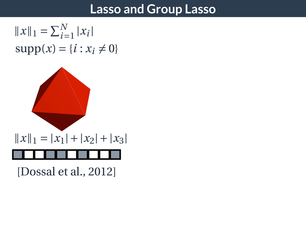
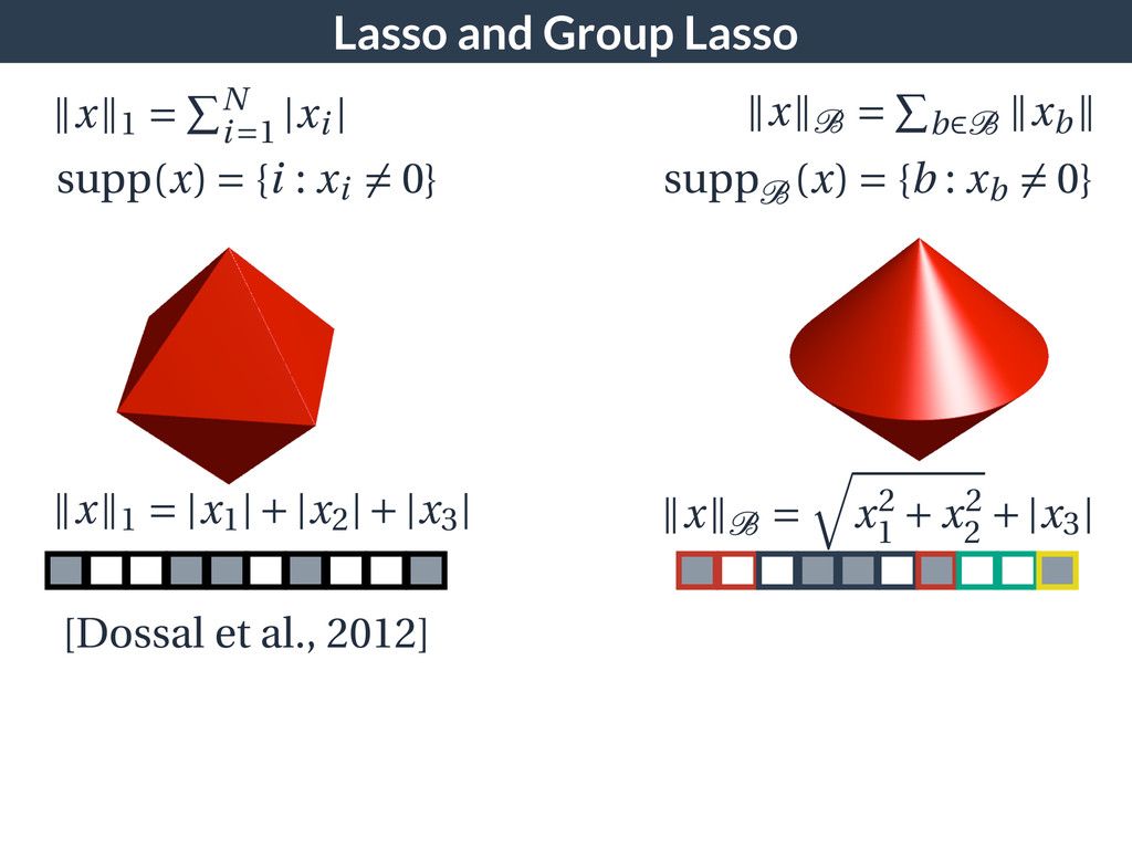
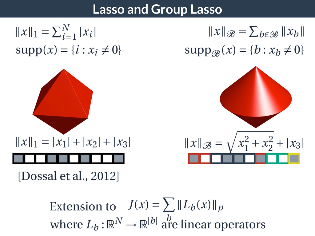
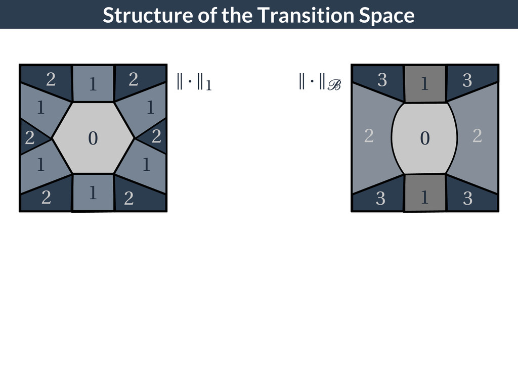
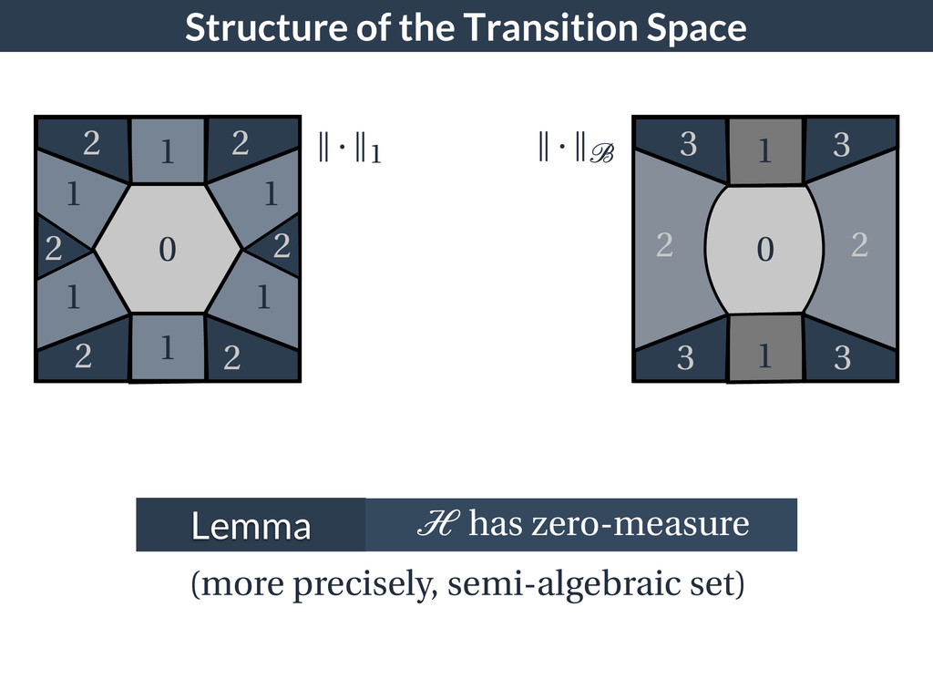
19. Lasso and Group Lasso supp(x) = {i : xi = 0} x 1 = |x1|+|x2|+|x3| x 1 = N i=1 |xi | x B = b∈B xb suppB (x) = {b : xb = 0} x B = x2 1 + x2 2 +|x3| J(x) = b Lb(x) p where Lb : RN R|b| are linear operators Extension to [Dossal et al., 2012]
20. Local Variations x(y) arg min x RN 1 2 y x 2 + J(x)
21. Local Variations x(y) arg min x RN 1 2 y x 2 + J(x) µ(y)= arg min x RN 1 2 y x 2 + J(x)
22. Local Variations x(y) arg min x RN 1 2 y x 2 + J(x) µ(y)= arg min x RN 1 2 y x 2 + J(x) Theorem y µ(y) is Lipschitz (hence weakly differentiable)
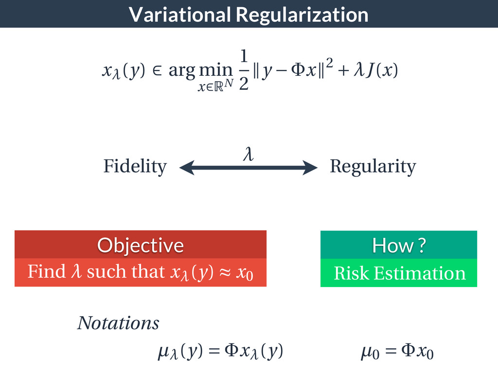
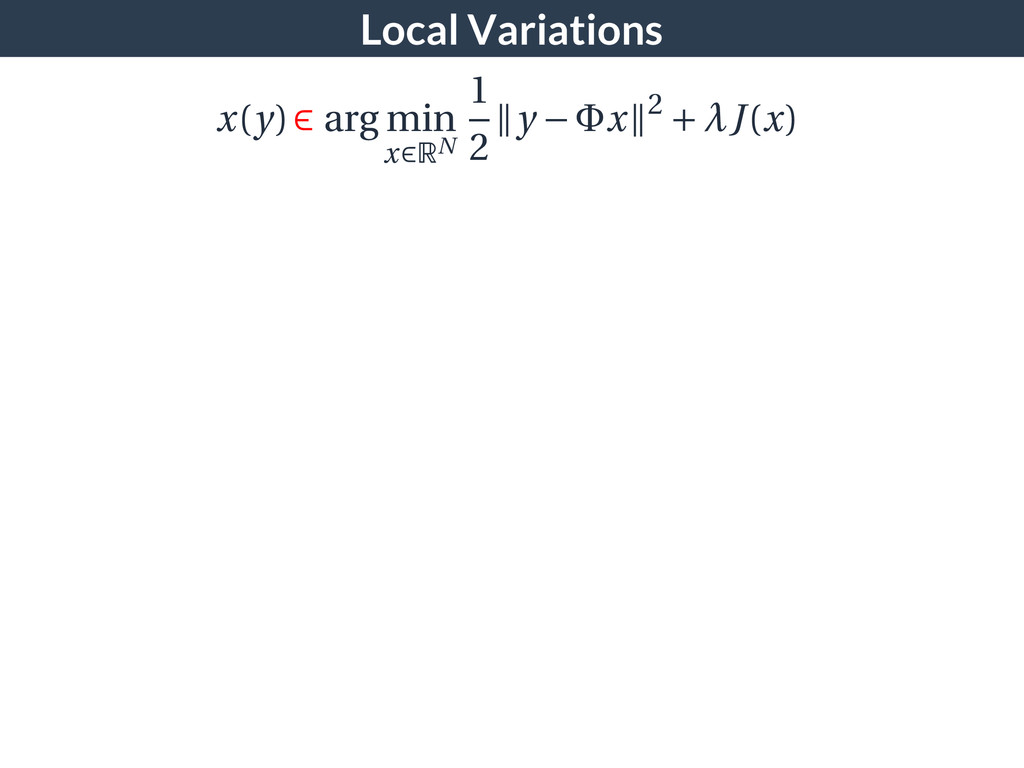
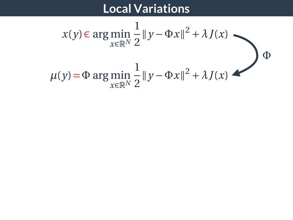
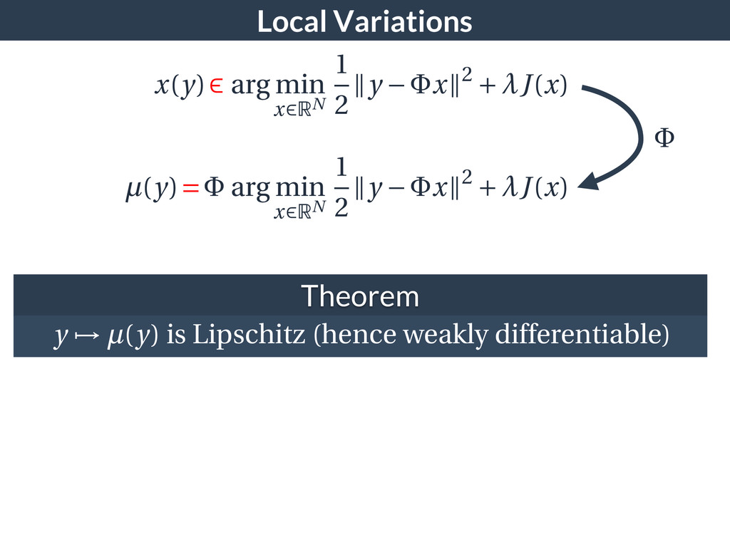
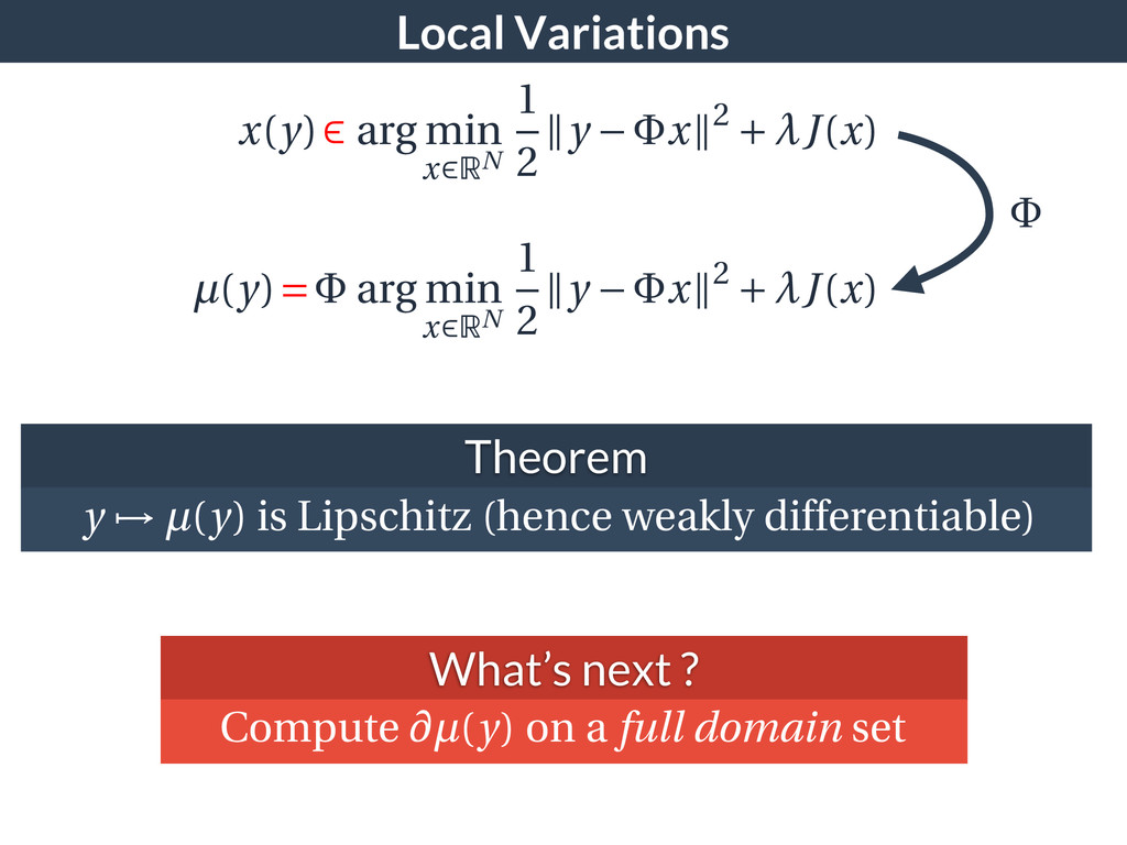
23. Local Variations x(y) arg min x RN 1 2 y x 2 + J(x) µ(y)= arg min x RN 1 2 y x 2 + J(x) Theorem y µ(y) is Lipschitz (hence weakly differentiable) What’s next ? Compute µ(y) on a full domain set
24. Local Support Constancy Lemma suppB (x( ¯ y)) = suppB (x(y)) for ¯ y close to y H .
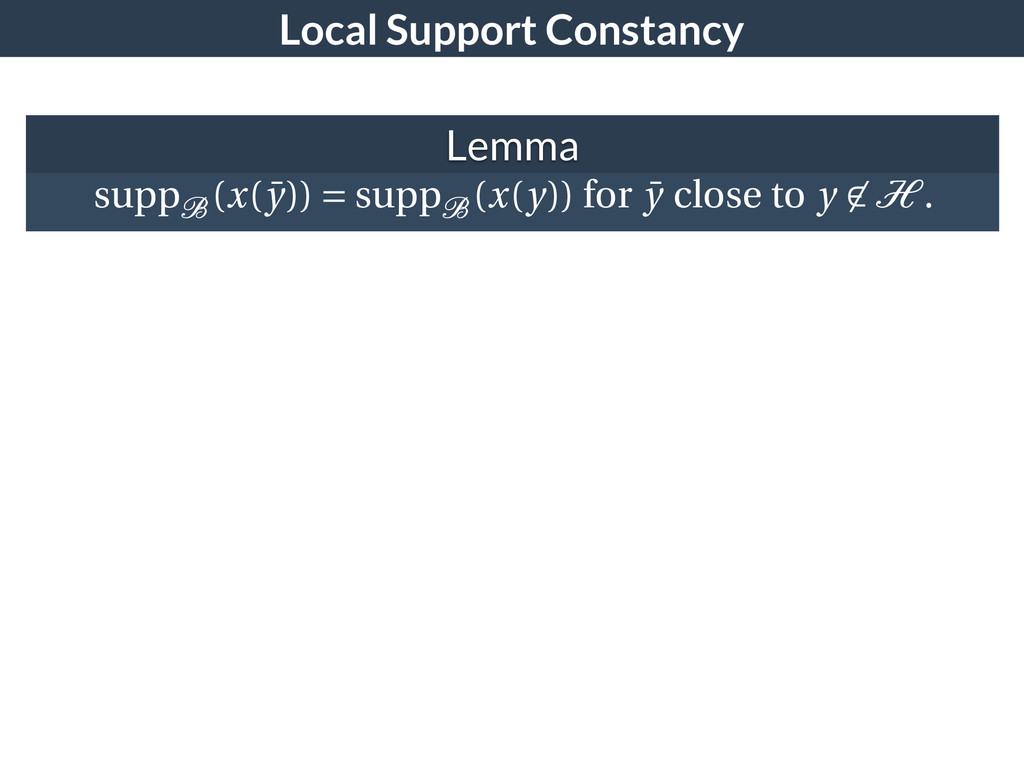
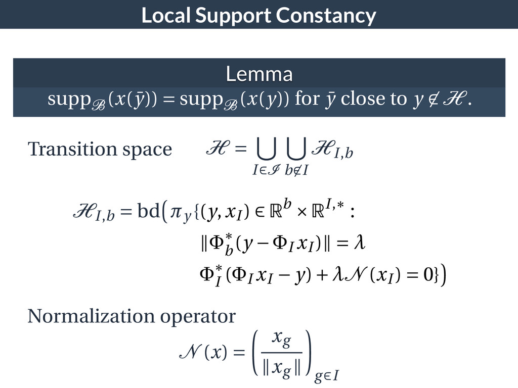
25. Local Support Constancy Lemma suppB (x( ¯ y)) = suppB (x(y)) for ¯ y close to y H . H = I I b I HI,b HI,b = bd y {(y,xI ) Rb RI, : b (y I xI ) = I ( I xI y)+ N (xI ) = 0} Normalization operator Transition space N (x) = xg xg g I
26. Structure of the Transition Space
27. Structure of the Transition Space · 1 0 1 1 1 1 1 1 2 2 2 2 2 2 · B 0 1 1 2 2 3 3 3 3
28. Structure of the Transition Space · 1 0 1 1 1 1 1 1 2 2 2 2 2 2 · B 0 1 1 2 2 3 3 3 3 Lemma H has zero-measure (more precisely, semi-algebraic set)
29. Differential Computation x( ¯ y) arg min x RN 1 2 ¯ y x 2 + J(x)
30. Differential Computation x( ¯ y) arg min x RN 1 2 ¯ y x 2 + J(x) First-order condition on I = suppB (x(y)) (xI ( ¯ y), ¯ y) = I ( I xI ( ¯ y) ¯ y)+ N (xI ( ¯ y))
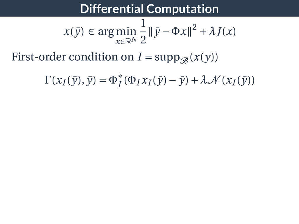
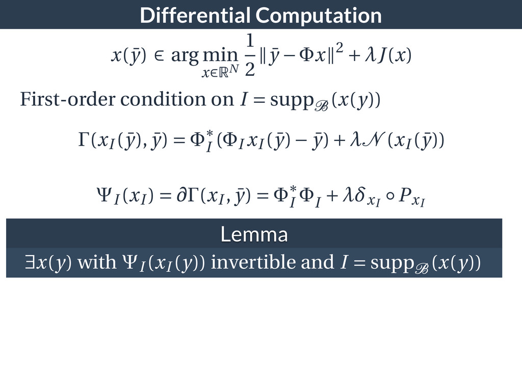
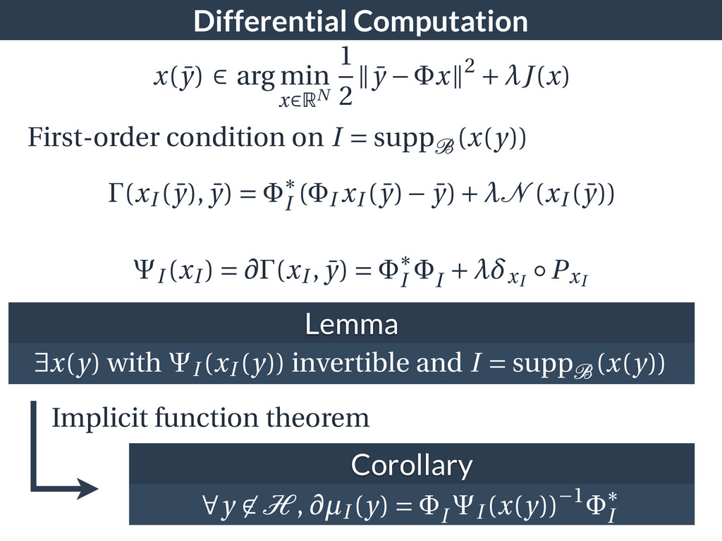
31. Differential Computation x( ¯ y) arg min x RN 1 2 ¯ y x 2 + J(x) I (xI ) = (xI , ¯ y) = I I + xI PxI Lemma x(y) with I (xI (y)) invertible and I = suppB (x(y)) First-order condition on I = suppB (x(y)) (xI ( ¯ y), ¯ y) = I ( I xI ( ¯ y) ¯ y)+ N (xI ( ¯ y))
32. Differential Computation x( ¯ y) arg min x RN 1 2 ¯ y x 2 + J(x) I (xI ) = (xI , ¯ y) = I I + xI PxI Lemma x(y) with I (xI (y)) invertible and I = suppB (x(y)) First-order condition on I = suppB (x(y)) (xI ( ¯ y), ¯ y) = I ( I xI ( ¯ y) ¯ y)+ N (xI ( ¯ y)) Corollary y H , µI (y) = I I (x(y)) 1 I Implicit function theorem
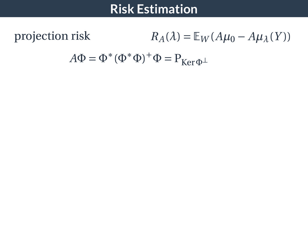
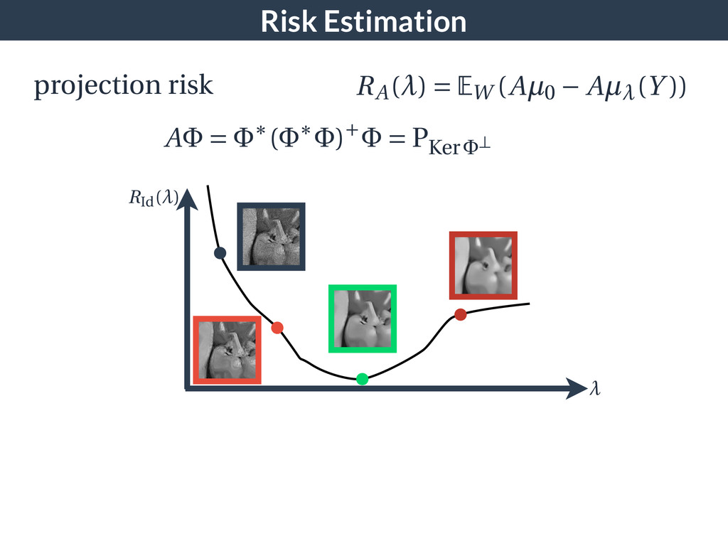
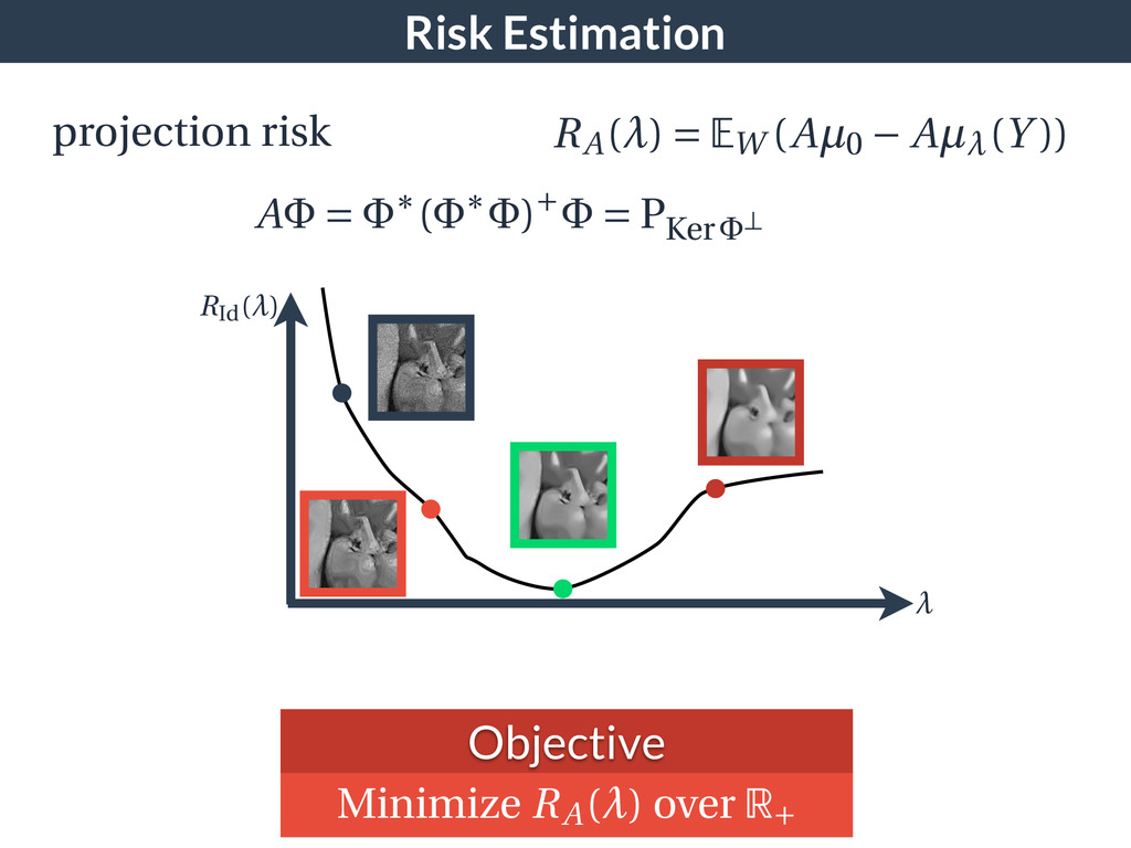
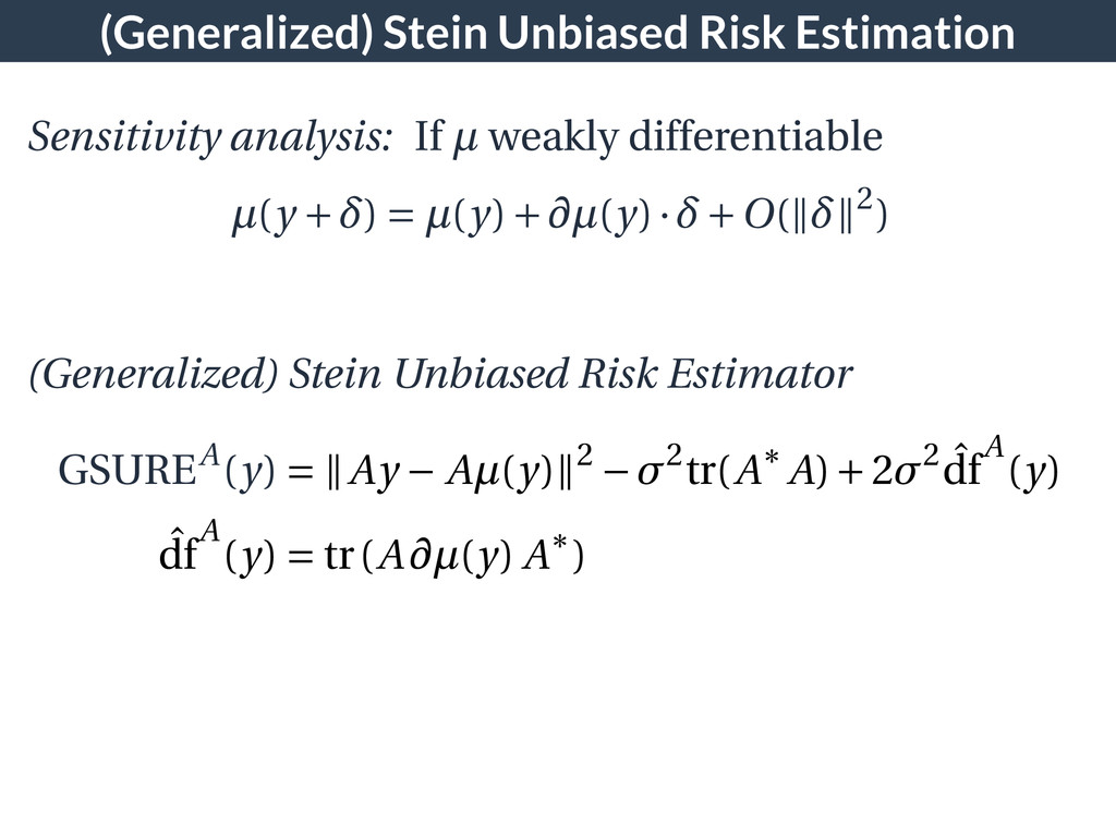
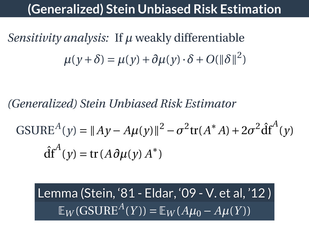
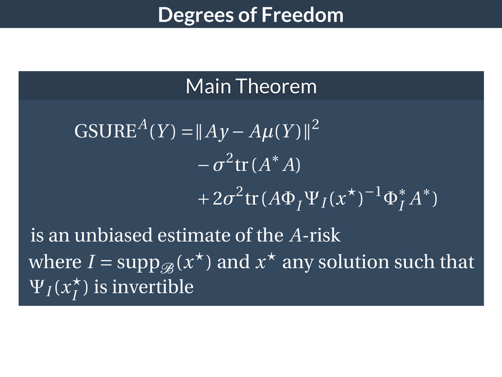
33. Degrees of Freedom Main Theorem where I = suppB (x ) and x any solution such that I (x I ) is invertible GSUREA(Y ) = Ay Aµ(Y ) 2 2tr(A A) +2 2tr(A I I (x ) 1 I A ) is an unbiased estimate of the A-risk
34. In Practice: Compressed Sensing : random CS matrix (ratio: 0.5) +y x opt (y) x0 J(x) = x B
35. In Practice: Tomography +y x opt (y) x0 J(x) = x B sub-sampled radon transform 16 measures
36. Conclusion sensitivity analysis risk estimation parameter selection
37. Conclusion Open Problems – Fast algorithms to compute – Extension to piecewise regular gauges sensitivity analysis risk estimation parameter selection