Low Complexity Regularizations: A ''Localization'' Result

Applied Inverse Problems 2015, Helsinki, May 2015

Transcript

1. Low Complexity Regularizations: a “Localization” Result Samuel Vaiter CMAP, École Polytechnique, France samuel.vaiter@cmap.polytechnique.fr Joint work with: Gabriel Peyré (CEREMADE, Univ. Paris–Dauphine) Jalal Fadili (GREY’C, ENSICAEN) May 29, 2015 AIP’15
2. Goal
3. Goal
4. Goal
5. Setting Linear inverse problem in finite dimension y = Φx0 + w Variational regularization (Tikhonov) x ∈ argmin x∈Rn 1 2 ||y − Φx||2 2 + λJ(x) (Pλ (y)) Noiseless constrained formulation x ∈ argmin x∈Rn J(x) subj. to y = Φx (P0 (y)) J convex, lower semicontinuous, proper function, typically non-smooth
6. Convex Prior sparsity ( 1 norm) J(x) = i |xi | small jump set (total variation) J(x) = max ξ∈K ξ, x spread representation ( ∞ norm) J(x) = max i |xi | low rank (trace/nuclear/1-Schatten/. . . norm) J(x) = i σi (x) sparse analysis (analysis 1 seminorm) J(x) = i | x, di |
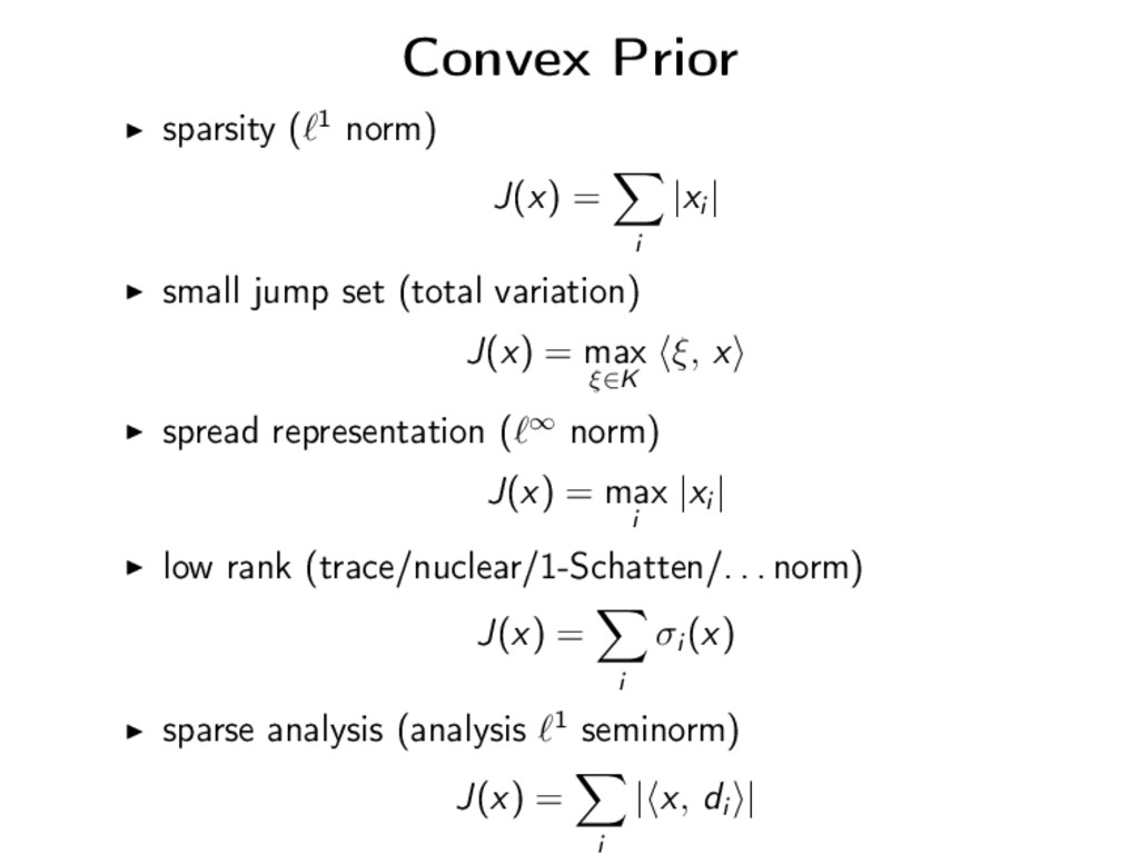
7. Toward a Unification Common properties: convex, lower semicontinuous, proper functions non-smooth promote objects which can be easily described Possible solutions: Union of subspaces Decomposable norm (Candes–Recht) Atomic norm (Chandrasekaran et al.) Decomposable prior (Negahban et al.)
9. Simple Observation The 1-norm is “almost”, “partially” smooth x x ∈ R2 with level-set || · ||1 x
10. Simple Observation The 1-norm is “almost”, “partially” smooth x x + δ x − δ x ∈ R2 with level-set || · ||1 x x + δ x − δ
11. Simple Observation The 1-norm is “almost”, “partially” smooth x x + δ x − δ x ∈ R2 with level-set || · ||1 x x + δ x − δ
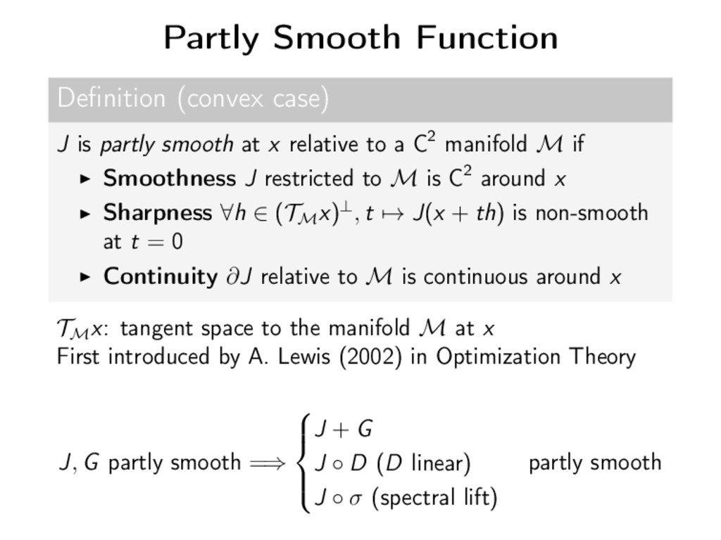
12. Partly Smooth Function Definition (convex case) J is partly smooth at x relative to a C2 manifold M if Smoothness J restricted to M is C2 around x Sharpness ∀h ∈ (TM x)⊥, t → J(x + th) is non-smooth at t = 0 Continuity ∂J relative to M is continuous around x TM x: tangent space to the manifold M at x First introduced by A. Lewis (2002) in Optimization Theory J, G partly smooth =⇒      J + G J ◦ D (D linear) J ◦ σ (spectral lift) partly smooth
13. Model Manifold Proposition The model manifold M is locally unique around x J = || · ||1 Mx = {z : supp(z) ⊆ supp(x)} J = ||∇ · ||1 Mx = {z : supp(∇z) ⊆ supp(∇x)} J = || · ||∗ Mx = {z : rank z = rank x} J = || · ||1,2 Mx = {z : suppB (z) ⊆ suppB (x)} J = || · ||1 + || · ||2 2 Mx = {z : supp(z) ⊆ supp(x)} J = || · ||2 Mx = Rn · · · Note: any decomposable or atomic norm is partly smooth
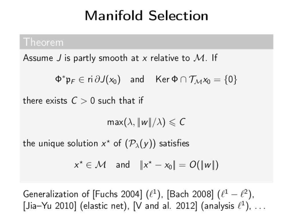
14. Manifold Selection Theorem Assume J is partly smooth at x relative to M. If Φ∗pF ∈ ri ∂J(x0 ) and Ker Φ ∩ TM x0 = {0} there exists C > 0 such that if max(λ, ||w||/λ) C the unique solution x of (Pλ (y)) satisfies x ∈ M and ||x − x0 || = O(||w||) Generalization of [Fuchs 2004] ( 1), [Bach 2008] ( 1 − 2), [Jia–Yu 2010] (elastic net), [V and al. 2012] (analysis 1), . . .
15. Linearized Pre-certificate Source condition / certificate Φ∗p ∈ ∂J(x0 ) Minimal norm certificate p0 = argmin ||p|| subj. to Φ∗p ∈ ∂J(x0 ) Linearized pre-certificate pF = argmin ||p|| subj. to Φ∗p ∈ aff ∂J(x0 )
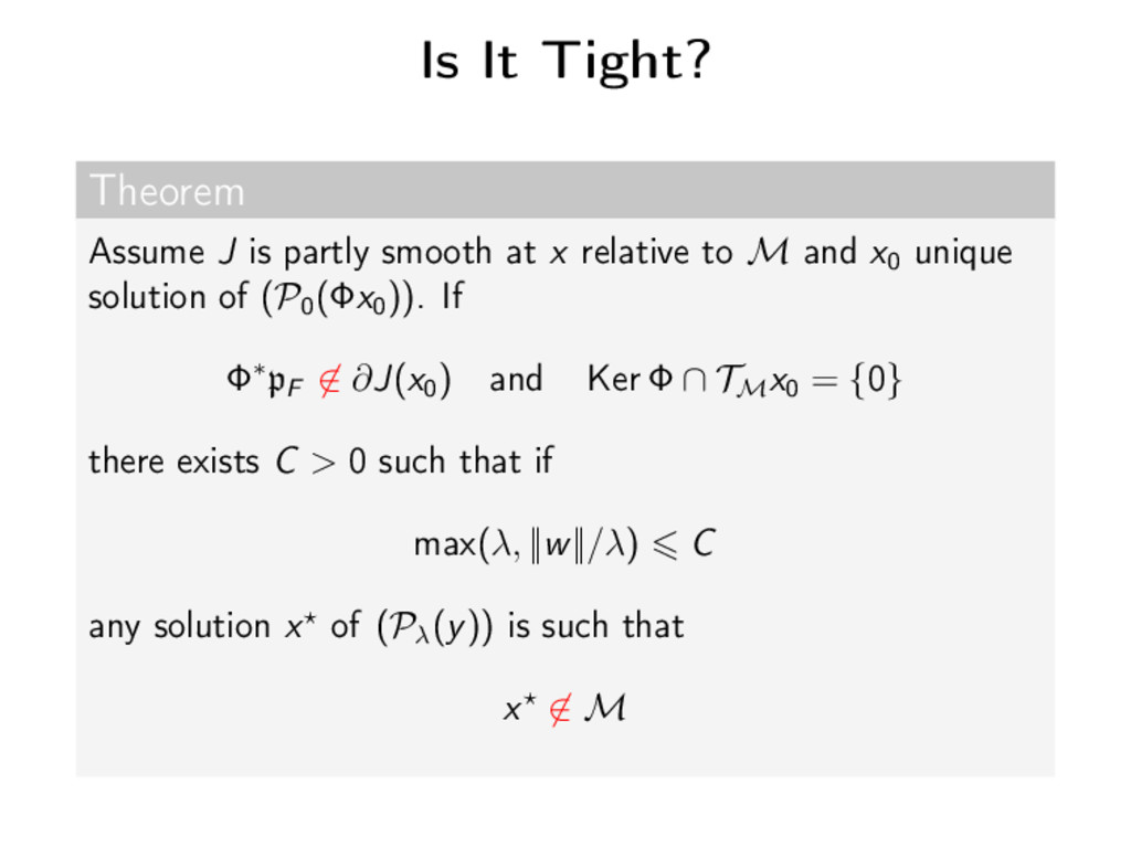
16. Is It Tight? Theorem Assume J is partly smooth at x relative to M and x0 unique solution of (P0 (Φx0 )). If Φ∗pF ∈ ∂J(x0 ) and Ker Φ ∩ TM x0 = {0} there exists C > 0 such that if max(λ, ||w||/λ) C any solution x of (Pλ (y)) is such that x ∈ M
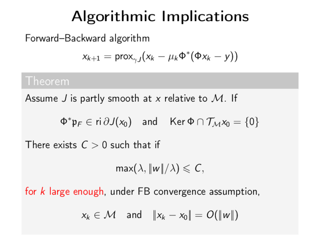
17. Algorithmic Implications Forward–Backward algorithm xk+1 = proxγJ (xk − µk Φ∗(Φxk − y)) Theorem Assume J is partly smooth at x relative to M. If Φ∗pF ∈ ri ∂J(x0 ) and Ker Φ ∩ TM x0 = {0} There exists C > 0 such that if max(λ, ||w||/λ) C, for k large enough, under FB convergence assumption, xk ∈ M and ||xk − x0 || = O(||w||)
18. 1D Total Variation and Jump Set J = ||∇d · ||1 , Mx = {x : supp(∇d x ) ⊆ supp(∇d x)} , Φ = Id i xi k uk stable jump +1 −1 unstable jump Φ∗pF = div u
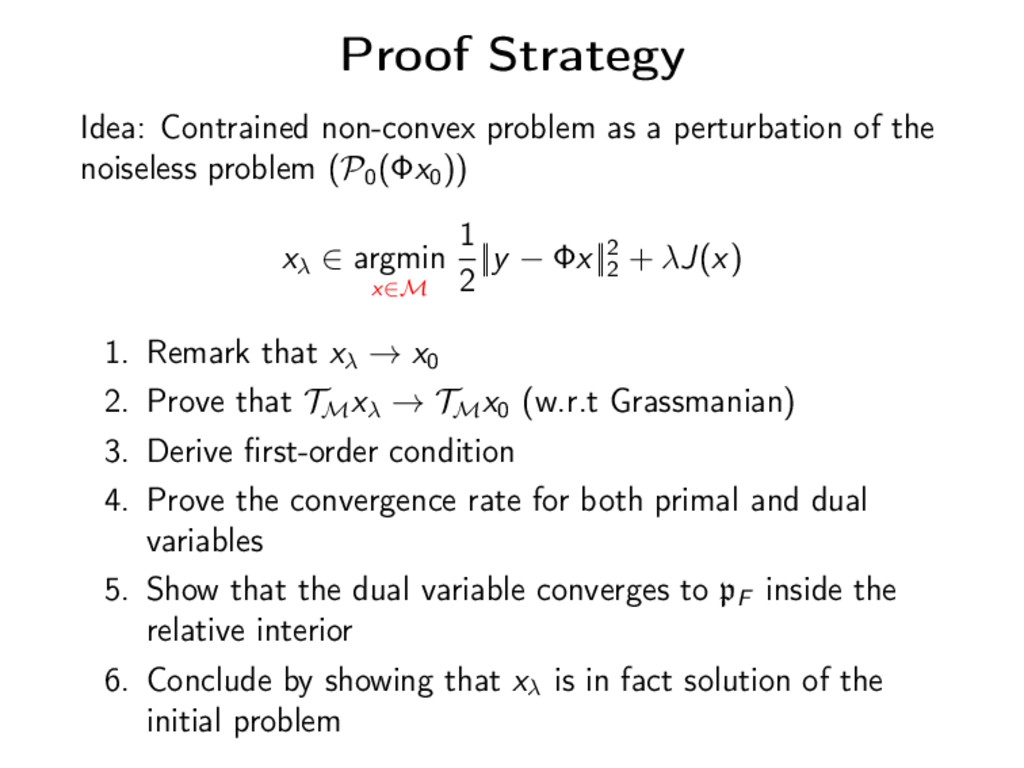
19. Proof Strategy Idea: Contrained non-convex problem as a perturbation of the noiseless problem (P0 (Φx0 )) xλ ∈ argmin x∈M 1 2 ||y − Φx||2 2 + λJ(x) 1. Remark that xλ → x0 2. Prove that TM xλ → TM x0 (w.r.t Grassmanian) 3. Derive first-order condition 4. Prove the convergence rate for both primal and dual variables 5. Show that the dual variable converges to pF inside the relative interior 6. Conclude by showing that xλ is in fact solution of the initial problem
20. Conclusion Signal models ←→ Singularities of J Combinatorial geometry Convex analysis Associated papers: SV, G. Peyré, and J. Fadili Model Consistency of Partly Smooth Regularizers SV, G. Peyré, and J. Fadili Low Complexity Regularization of Linear Inverse Problems Future work: Non-convex case & prior learning Infinite dimensional case: Radon measure: done (Duval & Peyré, 2015) Next step: Bounded variation . . .
21. Conclusion Signal models ←→ Singularities of J Combinatorial geometry Convex analysis Associated papers: SV, G. Peyré, and J. Fadili Model Consistency of Partly Smooth Regularizers SV, G. Peyré, and J. Fadili Low Complexity Regularization of Linear Inverse Problems Future work: Non-convex case & prior learning Infinite dimensional case: Radon measure: done (Duval & Peyré, 2015) Next step: Bounded variation . . . Thanks for your attention!