Dynamic Programming in Haskell

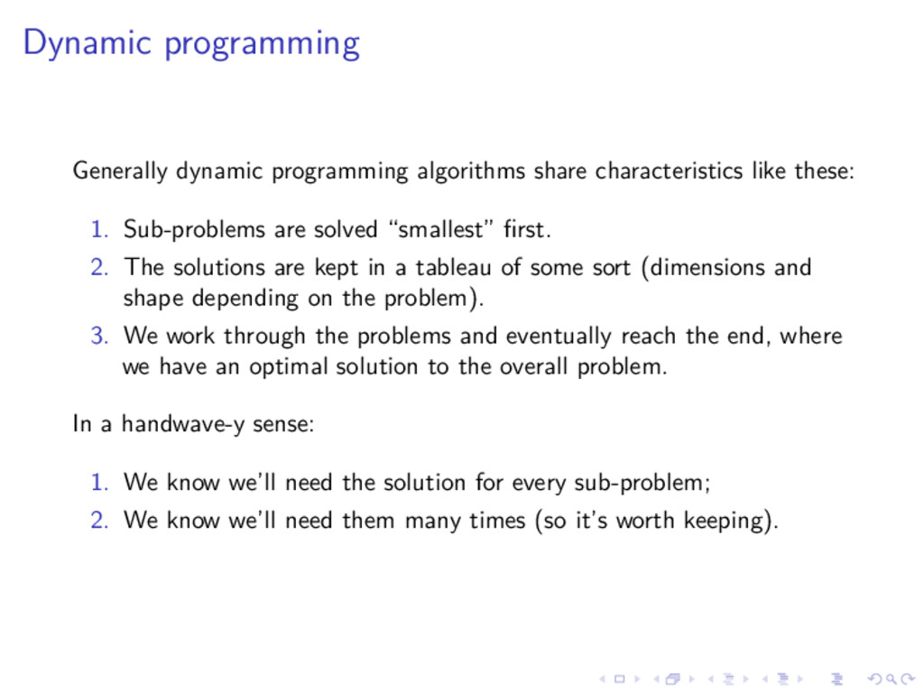
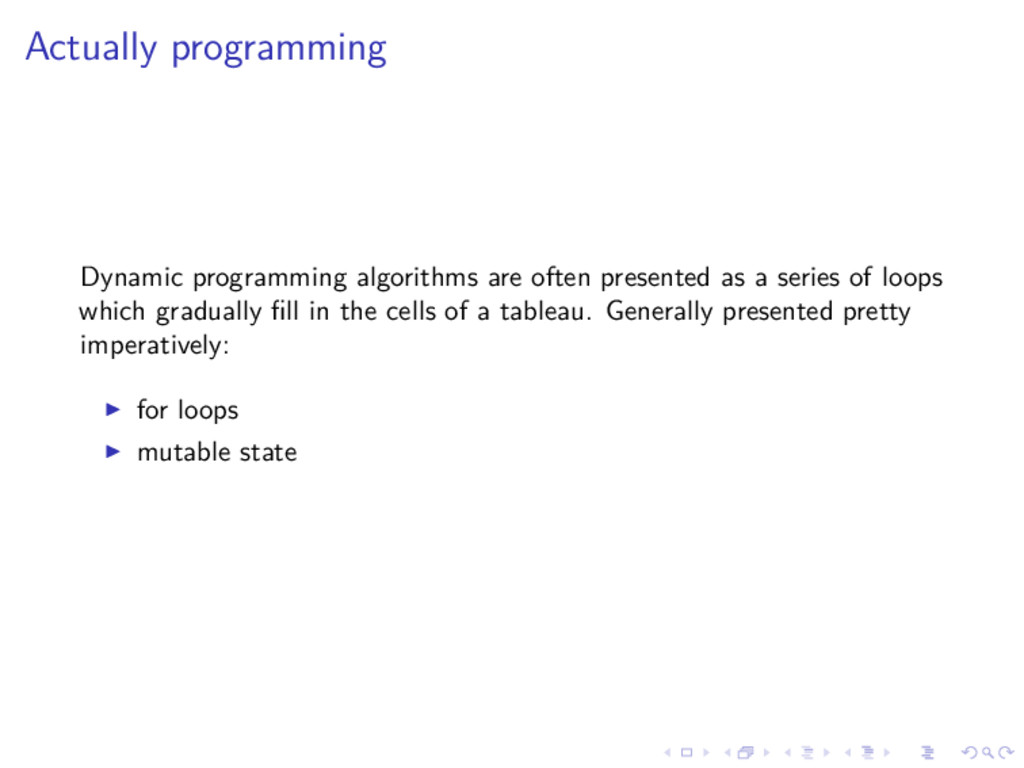
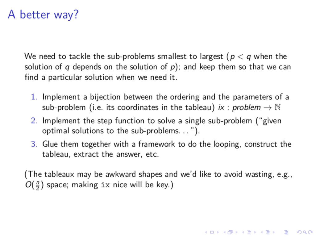
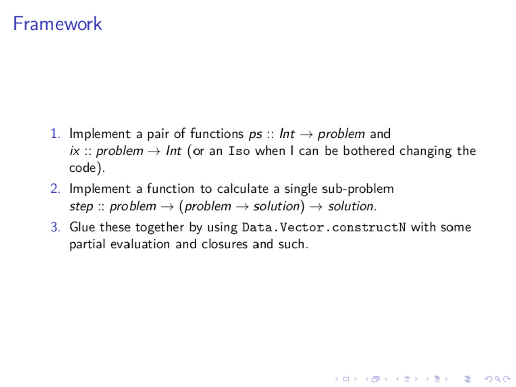
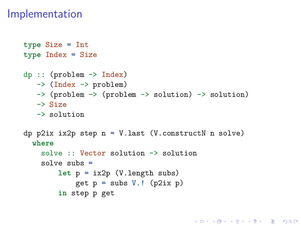
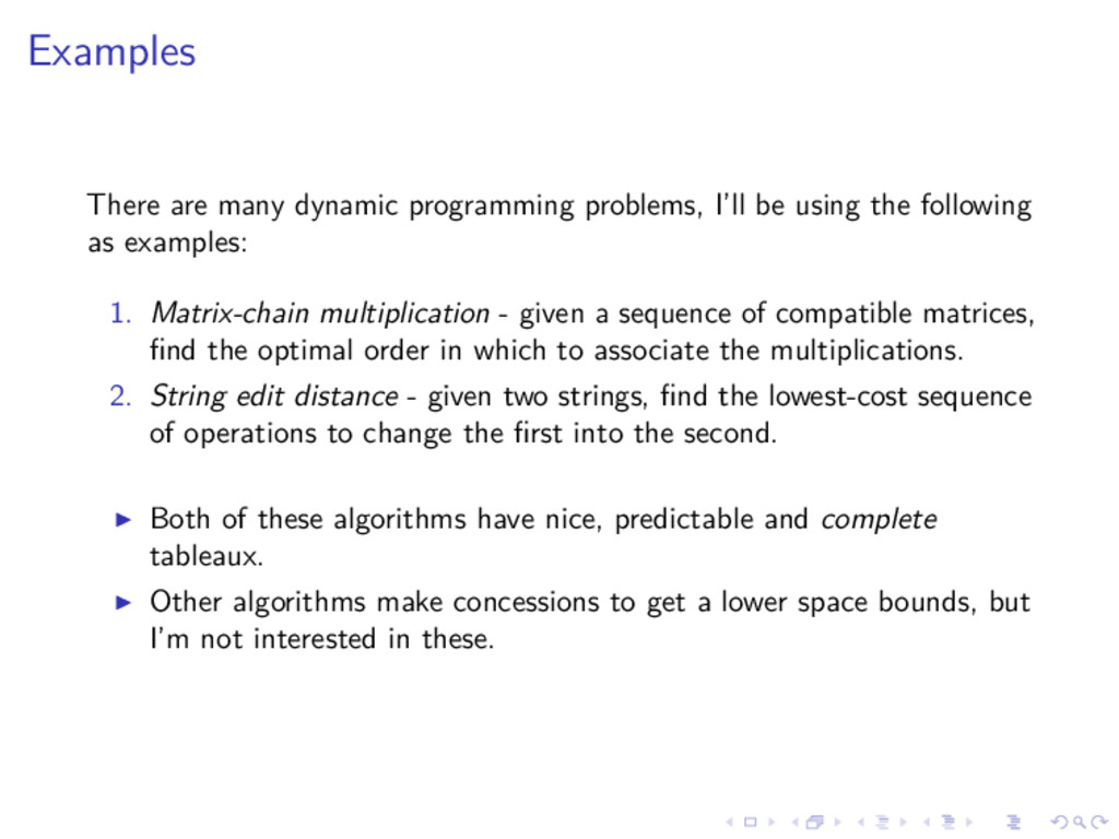
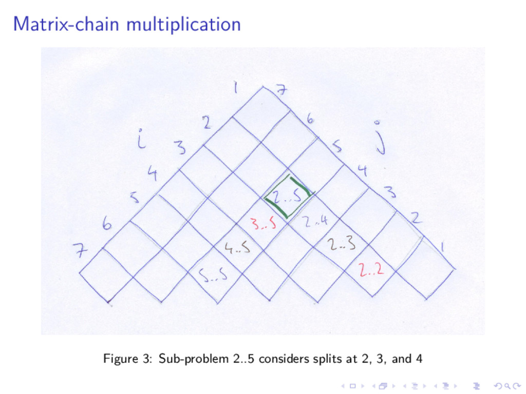
While textbooks and papers often present dynamic programming algorithms in an imperative style, there's usually nothing intrinsically imperative about them. In this talk I describe a framework for thinking about dynamic programming algorithms in a functional style and present two algorithms (matrix-chain multiplication and string edit distance) implemented in Haskell.

This presentation was delivered at the FP-Syd functional programming user group in Sydney, Australia in May, 2015.

Transcript

1. Dynamic Programming in Haskell Thomas Sutton, Anchor 2015-05-27
2. Introduction
3. Introduction This is a talk in two parts: 1. First I’ll introduce dynamic programming and a “framework” for implementing DP algorithms in Haskell using the vector library. 2. Second I’ll describe two algorithms and their implementation in this framework.
4. Dynamic Programming
5. Dynamic programming Dynamic programming is an approach to solving problems which exhibit two properties: Optimal substructure - an optimal solution can be found efficiently given optimal solutions to its sub-problems. Overlapping sub-problems - problems are divided into sub-problems which are used several times in the calculation of a solution to the overall problem. In practice this means: Solving a single “step” is efficient; and It’s worth keeping the solution to each step, because we’ll be reusing the answers a lot.
6. Dynamic programming Generally dynamic programming algorithms share characteristics like these: 1. Sub-problems are solved “smallest” first. 2. The solutions are kept in a tableau of some sort (dimensions and shape depending on the problem). 3. We work through the problems and eventually reach the end, where we have an optimal solution to the overall problem. In a handwave-y sense: 1. We know we’ll need the solution for every sub-problem; 2. We know we’ll need them many times (so it’s worth keeping).
7. Other approaches Dynamic programming can be contrasted with other approaches: Divide and conquer algorithms have sub-problems which do not necessarily overlap. Greedy algorithms work top-down selecting locally best sub-problems; so the solutions aren’t necessarily optimal. Memoisation algorithms maintain a cache past results so they can short-circuit when the same problem is solved in future.
8. Actually programming Dynamic programming algorithms are often presented as a series of loops which gradually fill in the cells of a tableau. Generally presented pretty imperatively: for loops mutable state
9. Actually programming MATRIX-CHAIN-ORDER(p) n <- length[p] - 1 for i <- 1 to n do m[i,i] <- 0 for l <- 2 to n do for i <- 1 to n - l + 1 do j <- i + l - 1 m[i,j] <- infinity for k <- i to j - 1 do q <- m[i,k] + m[k+1,j] + p[i-1] * p[k] * p[j] if q < m[i,j] do m[i,j] <- q s[i,j] <- k return m, s (From CLRS 2nd ed; p. 336)
10. Not actually imperative The key observation is that all these algorithms start with an empty tableau and gradually fill it in as they solve progressively larger sub-problems. The imperativeness is the only way they know how to do this. Poor them. :-(
11. A better way? We need to tackle the sub-problems smallest to largest (p < q when the solution of q depends on the solution of p); and keep them so that we can find a particular solution when we need it. 1. Implement a bijection between the ordering and the parameters of a sub-problem (i.e. its coordinates in the tableau) ix : problem → N 2. Implement the step function to solve a single sub-problem (“given optimal solutions to the sub-problems. . . ”). 3. Glue them together with a framework to do the looping, construct the tableau, extract the answer, etc. (The tableaux may be awkward shapes and we’d like to avoid wasting, e.g., O(n 2 ) space; making ix nice will be key.)
12. Framework 1. Implement a pair of functions ps :: Int → problem and ix :: problem → Int (or an Iso when I can be bothered changing the code). 2. Implement a function to calculate a single sub-problem step :: problem → (problem → solution) → solution. 3. Glue these together by using Data.Vector.constructN with some partial evaluation and closures and such.
13. Implementation type Size = Int type Index = Size dp :: (problem -> Index) -> (Index -> problem) -> (problem -> (problem -> solution) -> solution) -> Size -> solution dp p2ix ix2p step n = V.last (V.constructN n solve) where solve :: Vector solution -> solution solve subs = let p = ix2p (V.length subs) get p = subs V.! (p2ix p) in step p get
14. Example problems
15. Examples There are many dynamic programming problems, I’ll be using the following as examples: 1. Matrix-chain multiplication - given a sequence of compatible matrices, find the optimal order in which to associate the multiplications. 2. String edit distance - given two strings, find the lowest-cost sequence of operations to change the first into the second. Both of these algorithms have nice, predictable and complete tableaux. Other algorithms make concessions to get a lower space bounds, but I’m not interested in these.
16. Matrix-chain multiplication
17. Matrix-chain multiplication Matrix multiplication is a pretty big deal. Assuming you have two matrices with dimensions A1 : m × n and A2 : n × o then multiplying them will take O(m × n × o) scalar operations (using the naive algorithm). Matrix multiplication is associative (but not commutative) so we can “bracket” a chain of n > 2 matrices however we like. The matrix-chain multiplication problem is to choose the best (i.e. least cost) way to bracket a matrix multiplication chain. First, let’s see why we need an algorithm?
18. Example: Multiply three matrices A1 : 10 × 100 A2 : 100 × 5 A3 : 5 × 50 There are two ways we can evaluate the chain A1 A2 A3 : (A1 A2 )A3 or A1 (A2 A3 ). (A1 A2 )A3 = (10 × 100 × 5) + (10 × 5 × 50) = 7500 A1 (A2 A3 ) = (10 × 100 × 50) + (100 × 5 × 50) = 75000 We’ve only had to make one choice and we’ve already done, potentially, an order of magnitude too much work!
19. Matrix-chain multiplication Suppose we have a chain Ai Ai+1 Ai+2...Ai+n of n matrices we wish to multiply. Any solution splits the chain in two – a left side and a right side – which must each be multiplied out before multiplying the results together. We are free to split at any point j in the chain 1 < j < n. The left and right sides are both sub-problems.
20. Matrix-chain multiplication 1. For all possible splitting points s: 1.1 Calculate the cost of the right sub-problem; and 1.2 Calculate the cost of the left sub-problem. 2. Solve the problem by choosing the splitting point s to minimise: 2.1 The cost of the left sub-problem Ai ..Ai+s ; and 2.2 The cost of the right sub-problem Ai+s+1..Ai+n ; and 2.3 The cost of multiplying the solutions of the two sub-problems together. In (1) we’re calculating the solutions to all sub-problems and in (2) we’re choosing and combining the optimal sub-problems into an optimal solution. A recursive implementation results in an enormous amount of repeated work, so we’ll use a dynamic algorithm.
21. Matrix-chain multiplication The key is a tableau which holds the intermediate sub-problems: Figure 1: Empty MCM tableau
22. Matrix-chain multiplication Figure 2: Sub-problem 3..5 considers splits at 3 and 4
23. Matrix-chain multiplication Figure 3: Sub-problem 2..5 considers splits at 2, 3, and 4
24. Matrix-chain multiplication A solution (Int, (Int, Int), Vector Int) includes the number of scalar multiplications, dimensions of the resulting matrix, and splitting points. For a chain of n matrices the vector is n∗(n+1) 2 long (this is the nth triangular number). We map between the tableau and the vector a little trickily: ix :: Size -> Problem -> Index ix n (i,j) = let x = n - j + i + 1 in i + (n * (n-1) div 2) - ((x-1) * x div 2) param :: Size -> Index -> Problem param n x = -- (ix n (i,j) = x), solve for (i,j)
25. Matrix-chain multiplication solve ms (i,j) get -- Sub-problem of length = 1. | i == j = (0, ms V.! i, mempty) -- Sub-problem of length > 1; check the possible splits. | otherwise = minimumBy (compare on fsst) $ map subproblem [i..j-1] where subproblem s = let (lc, (lx,ly), ls) = get (i,s) (rc, ( _,ry), rs) = get (s+1,j) in ( lc + rc + (lx * ly * ry) , (lx, ry) , V.singleton s <> ls <> rs )
26. Matrix-chain multiplication -- | Solve a matrix-chain multiplication problem. mcm :: Vector (Int,Int) -> (Int, (Int,Int), Vector Int) mcm ms = let n = V.length ms in dp (ix n) (param n) (solve ms) (triangularNumber n)
27. String edit distance
28. String edit distance Given two strings, find the optimal cost (and/or the sequence of operations) to transform the first string into the latter. We aren’t committed to any particular set of operations but we’ll use: Insert: cost(cat → chat) = 1 Delete: cost(cat → ca) = 1 Substitute: cost(cat → sat) = 1
29. String edit distance The tableau for a string edit distance problem is a little simpler, it’s just an n × m matrix for “from” and “to” strings of n and m symbols: s a t u r d a y c a t (Well actually, it’s (n + 1) × (m + 1).)
30. String edit distance The sub-problem structure here comes from the prefix structure of the strings themselves. Given some optimal solution for cost(s → t), we can solve: Extend: cost(s c → t c) = cost(s → t) Delete: cost(s c → t) = cost(s → t) + delete Insert: cost(s → t c) = cost(s → t) + insert Substitute: cost(s c → t d) = cost(s → t) + subst
31. String edit distance The trivial cases in string edit distance are a tiny bit less trivial than for MCM: s a t u r d a y 0 1 2 3 4 5 6 7 8 c 1 a 2 t 3
32. String edit distance Filling in the rest of the tableau is pretty straightforward: if s[x] == t[y] then m[x,y] <- m[x-1,y-1] -- Nop: + 0 else m[x,y] <- min { m[x-1,y ] + 1 -- Ins: ← + 1 , m[x ,y-1] + 1 -- Del: ↑ + 1 , m[x-1,y-1] + 1 -- Sub: + 1 }
33. String edit distance s a t u r d a y 0 1 2 3 4 5 6 7 8 c 1 1 2 3 4 5 6 7 8 a 2 2 ? t 3 s[y] = t[x] so no edit operation required, this is an extension: m[x, y] ← m[x − 1, y − 1].
34. String edit distance s a t u r d a y 0 1 2 3 4 5 6 7 8 c 1 1 2 3 4 5 6 7 8 a 2 2 1 ? t 3 s[y] = t[x] so we check the cases: Insert “t”: m[x − 1, y] + 1 Delete “a”: m[x, y − 1] + 1 Replace “a” with “t”: m[x − 1, y − 1] + 1 We choose the least: m[x, y] ← m[x − 1, y] + 1.
35. String edit distance We can the cost from the cell m[len(t), len(s)] or follow the path back through the tableau to determine an edit script. s a t u r d a y 0 1 2 3 4 5 6 7 8 c 1 1 2 3 4 5 6 7 8 a 2 2 1 2 3 4 5 6 7 t 3 3 2 1 2 3 4 5 6 This is usually called Wagner-Fischer algorithm and about a dozen other things.
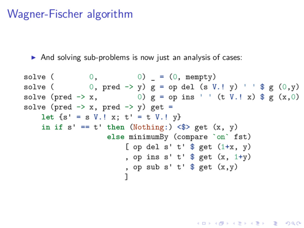
36. Wagner-Fischer algorithm We’ll find (Int, [Op]) solutions which include the lowest cost and the edit script for the optimal solution. The vector is n × m long, each value depends only on cells before it in the ordering. We map the n × m tableau to a Vector in the obvious way: ix :: Size -> Problem -> Index ix n (x,y) = (x * n) + y param :: Size -> Index -> Problem param n i = i quotRem n
37. Wagner-Fischer algorithm And solving sub-problems is now just an analysis of cases: solve ( 0, 0) _ = (0, mempty) solve ( 0, pred -> y) g = op del (s V.! y) $ g (0,y) solve (pred -> x, 0) g = op ins (t V.! x) $ g (x,0) solve (pred -> x, pred -> y) get = let {s = s V.! x; t = t V.! y} in if s == t then (Nothing:) <$> get (x, y) else minimumBy (compare on fst) [ op del s t $ get (1+x, y) , op ins s t $ get (x, 1+y) , op sub s t $ get (x,y) ]
38. Wagner-Fischer algorithm Gluing these bits together we get: editDistance :: Vector Char -> Vector Char -> Solution editDistance s t = (reverse . catMaybes) <$> let {m = V.length s; n = V.length t} in dp (ix n) (param n) solve (m * n)
39. Conclusion
40. Conclusions Dynamic programming is a great and fits naturally into standard libraries in the Haskell ecosystem. The mutation used in the descriptions of many algorithms is often incidental; you can probably find a way to remove it or hide it behind an API. Finding a suitable isomorphism Index ↔ problem which orders sub-problems appropriately is the key; if you care about complexity analysis of the whole algorithm this should probably be O(1). (Finding an appropriate O(1) bijections between indexes in a funny-shaped matrix and N can be tricky, especially if you can’t remember high-school algebra.)