3/16
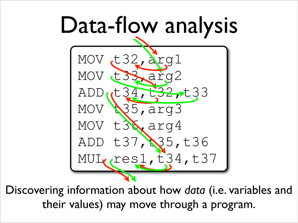
* Data-flow analysis collects information about how data moves through a program
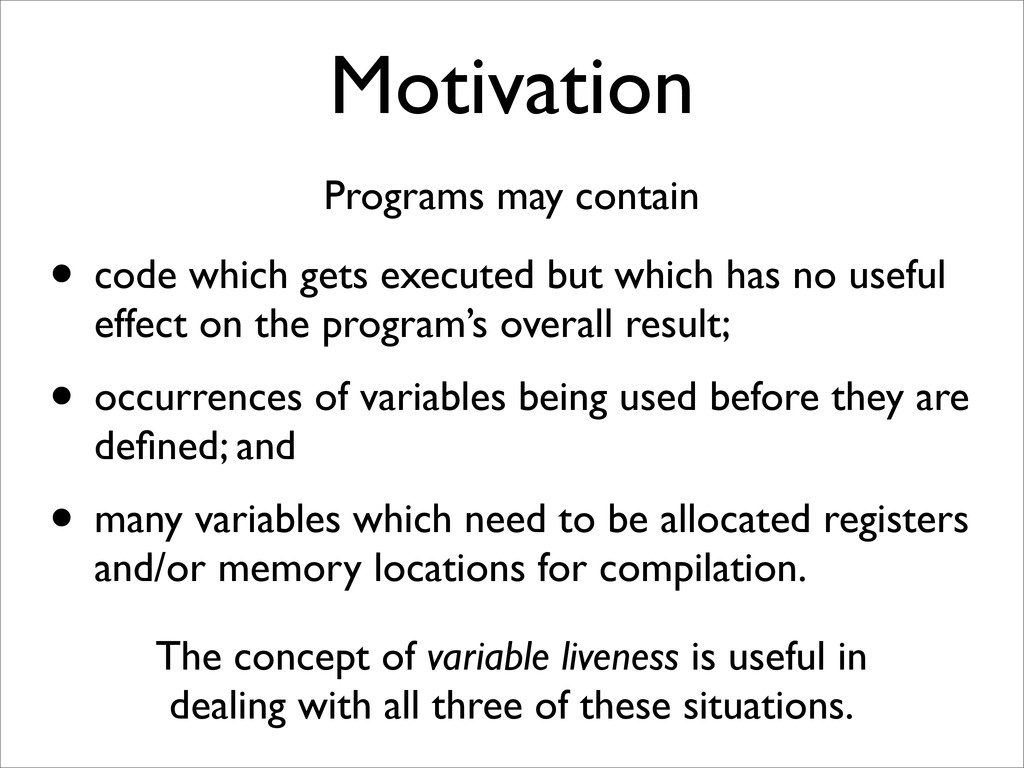
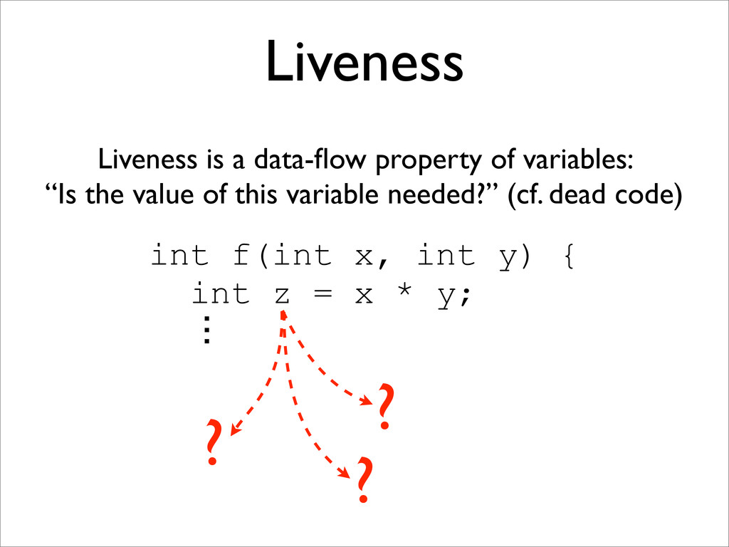
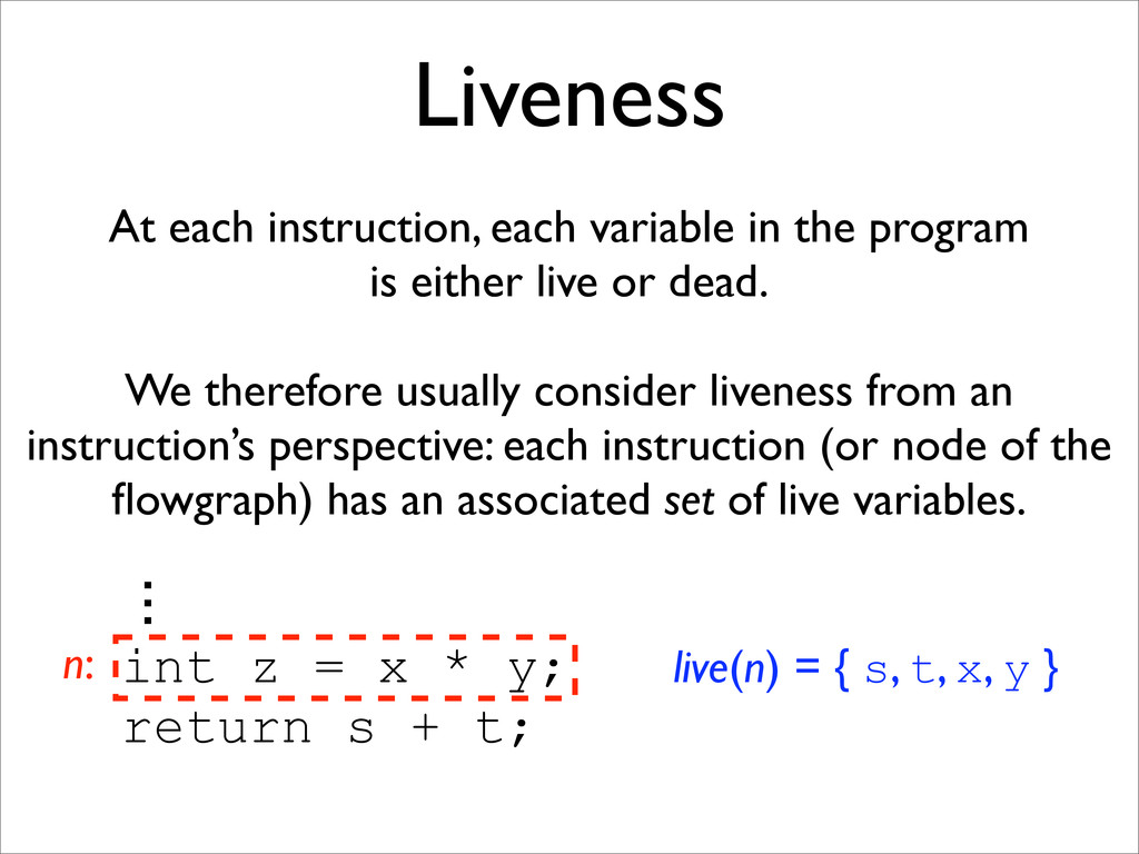
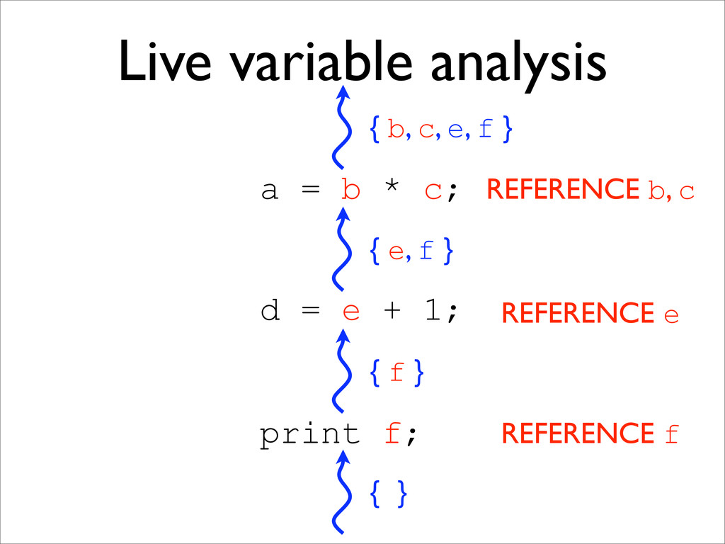
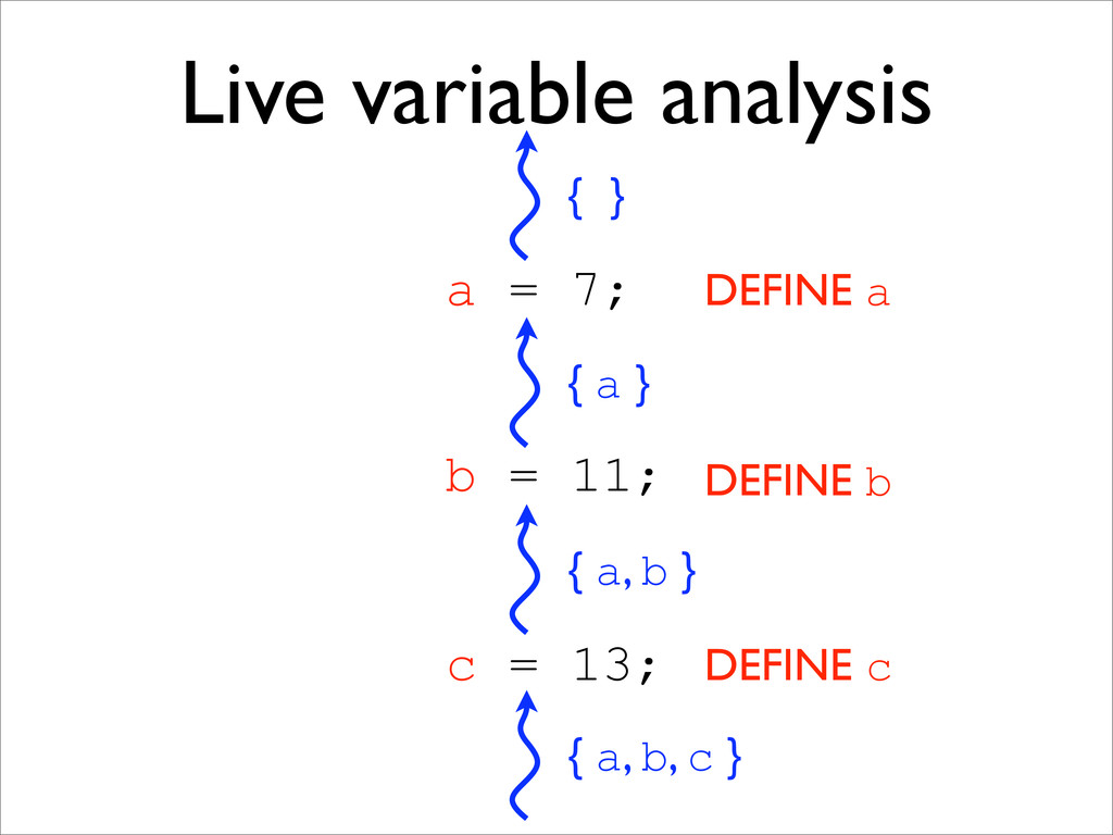
* Variable liveness is a data-flow property
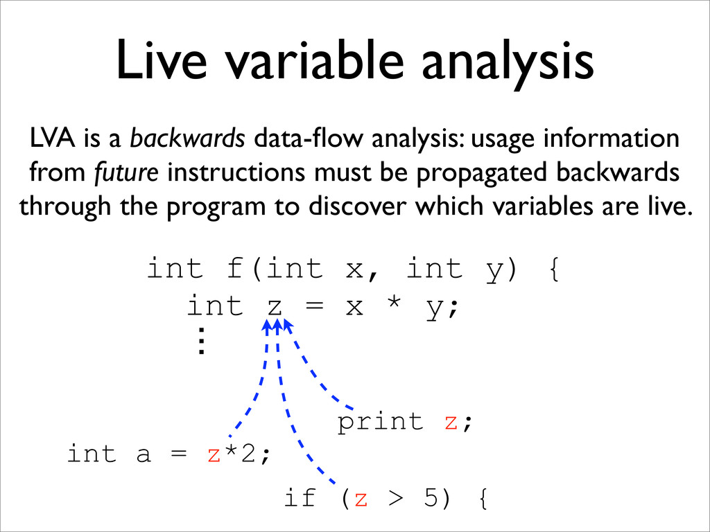
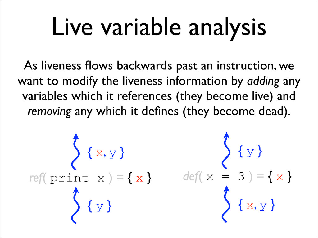
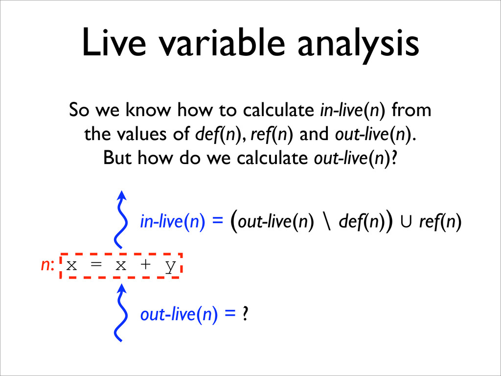
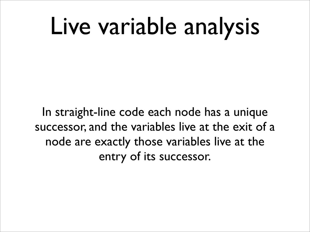
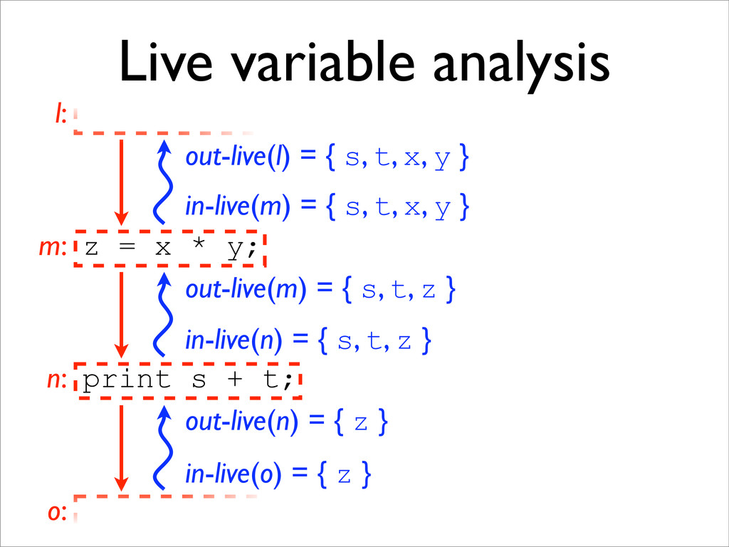
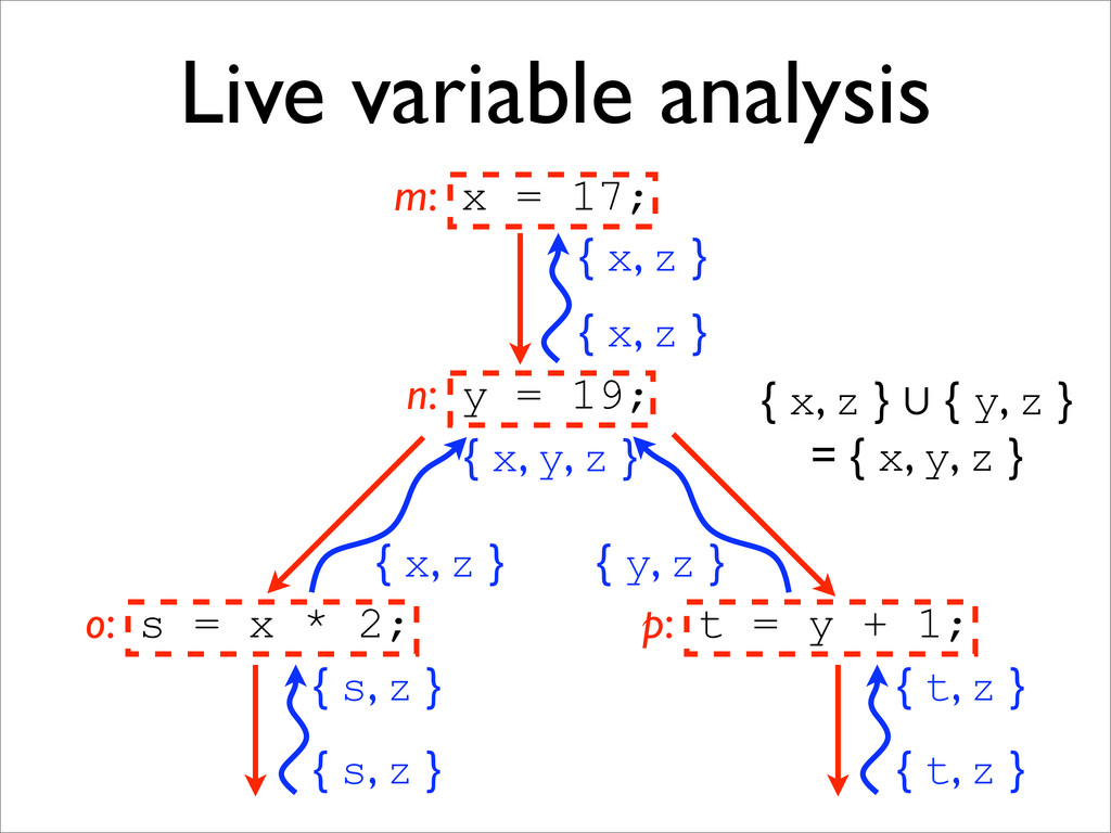
* Live variable analysis (LVA) is a backwards data-flow analysis for determining variable liveness
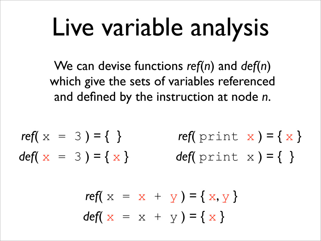
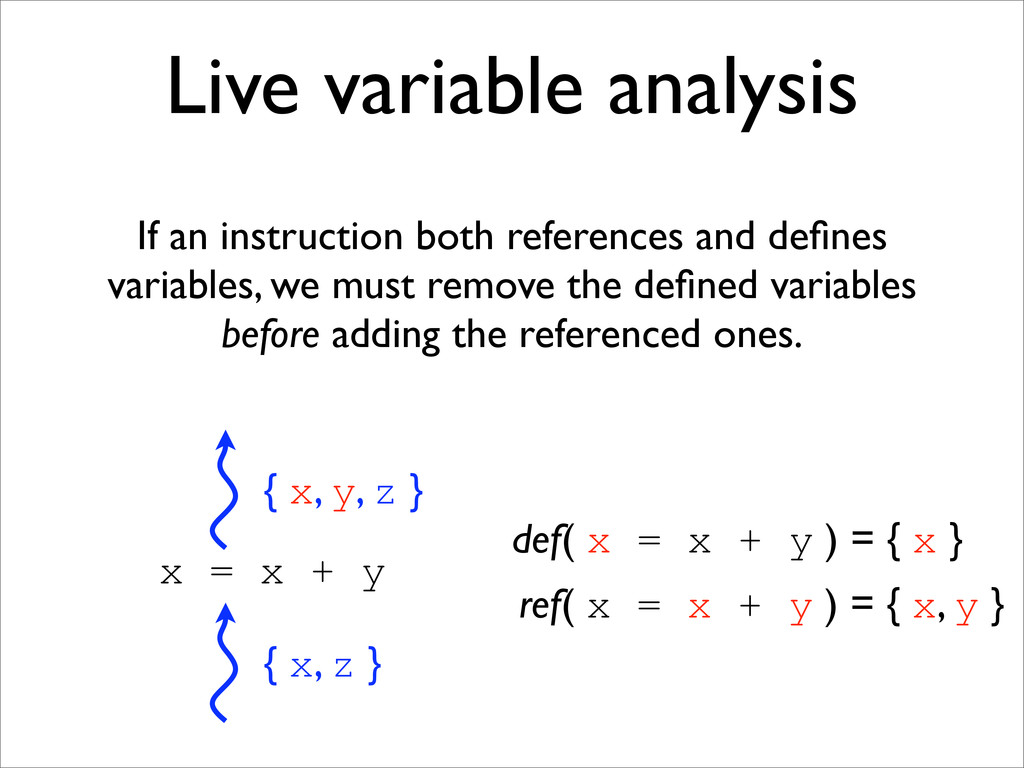
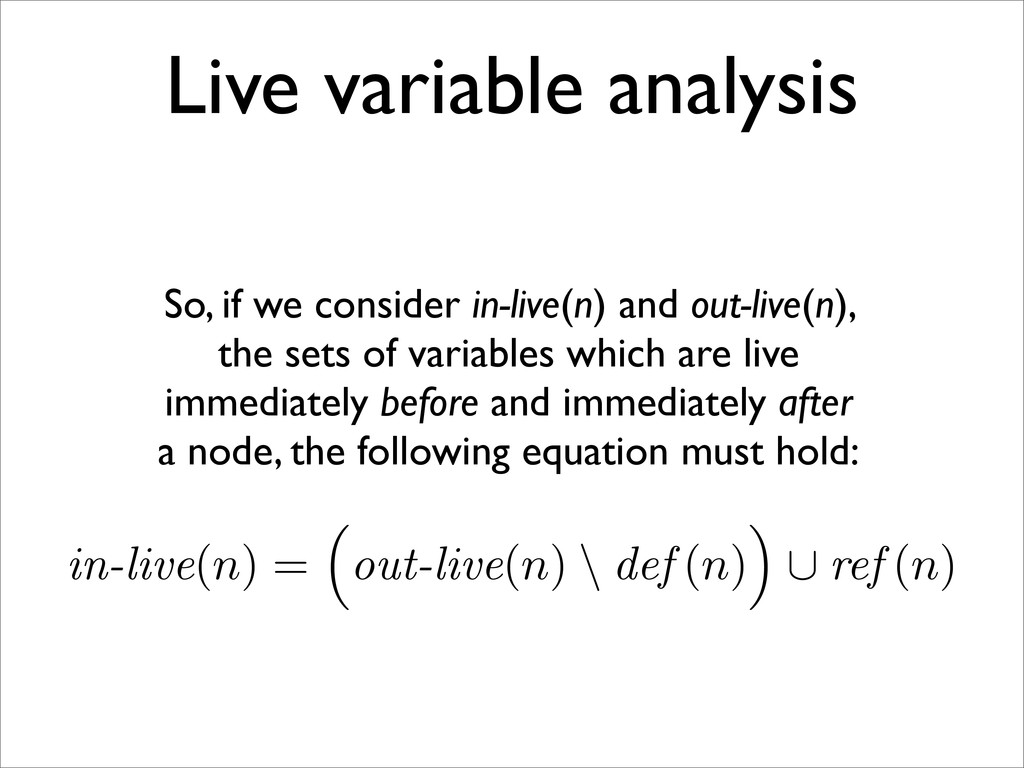
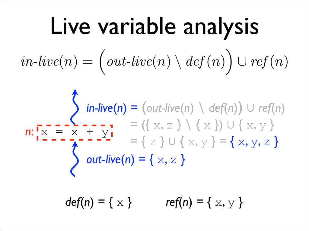
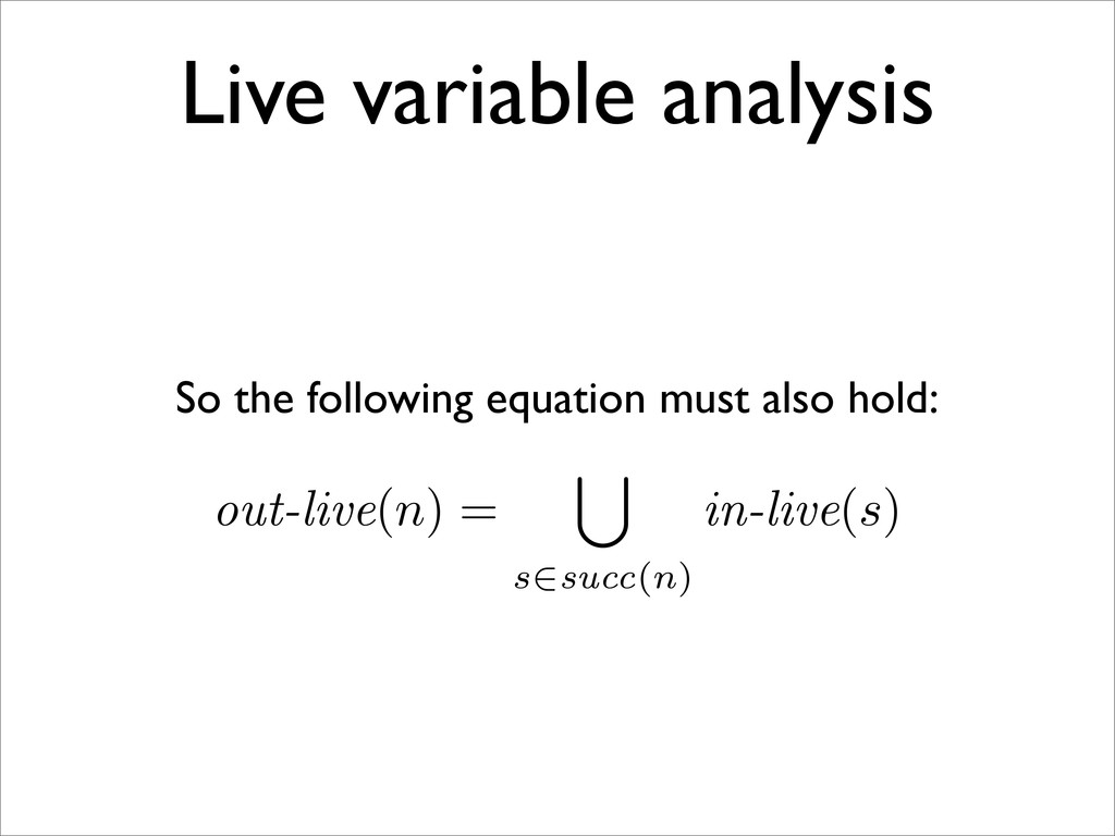
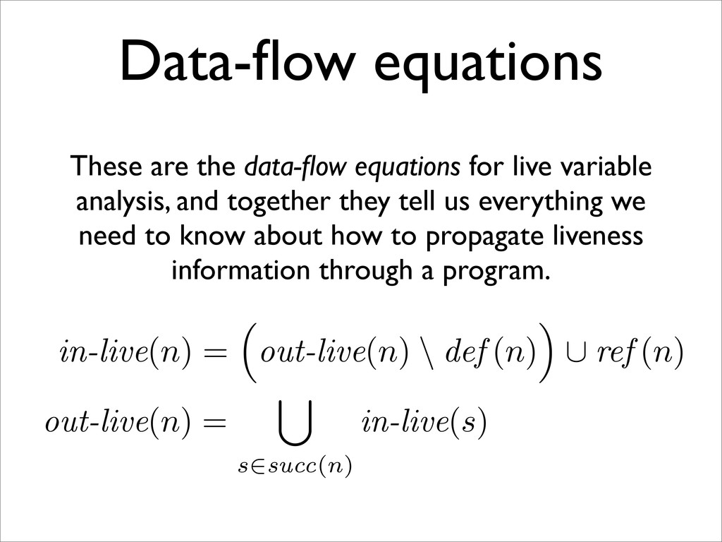
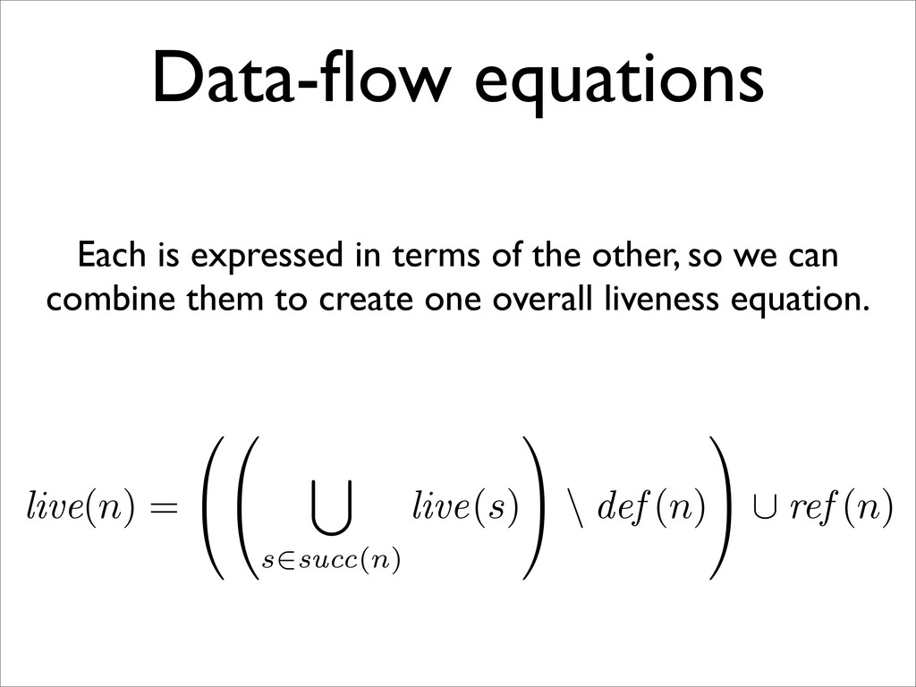
* LVA may be expressed as a pair of complementary data-flow equations, which can be combined
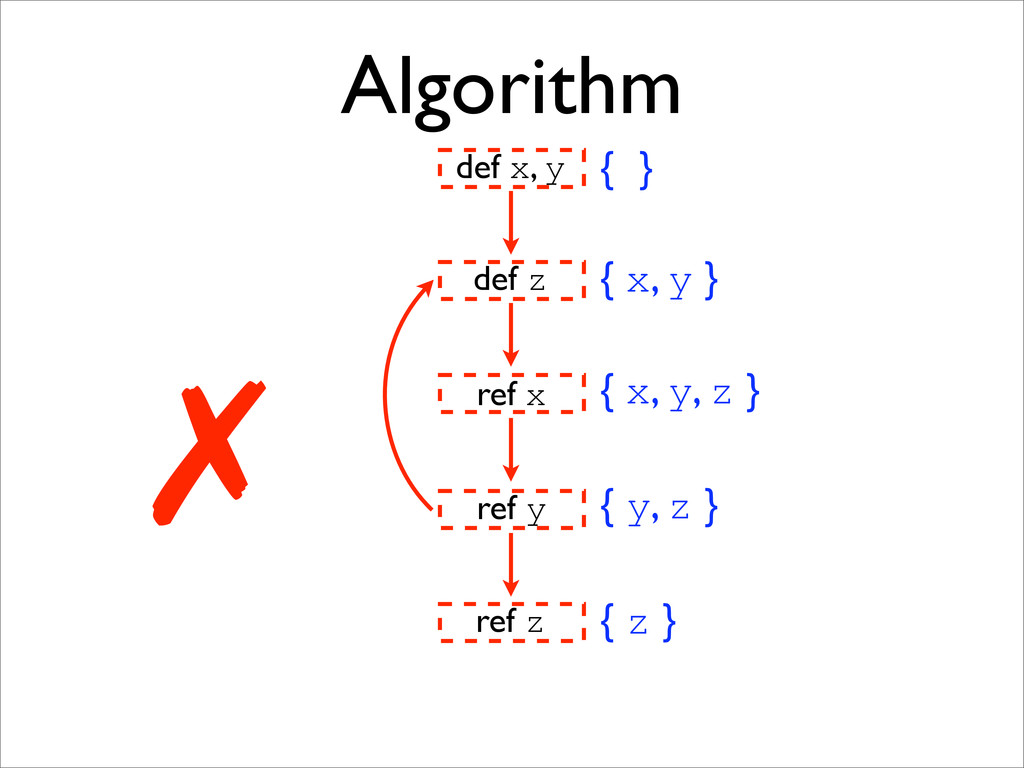
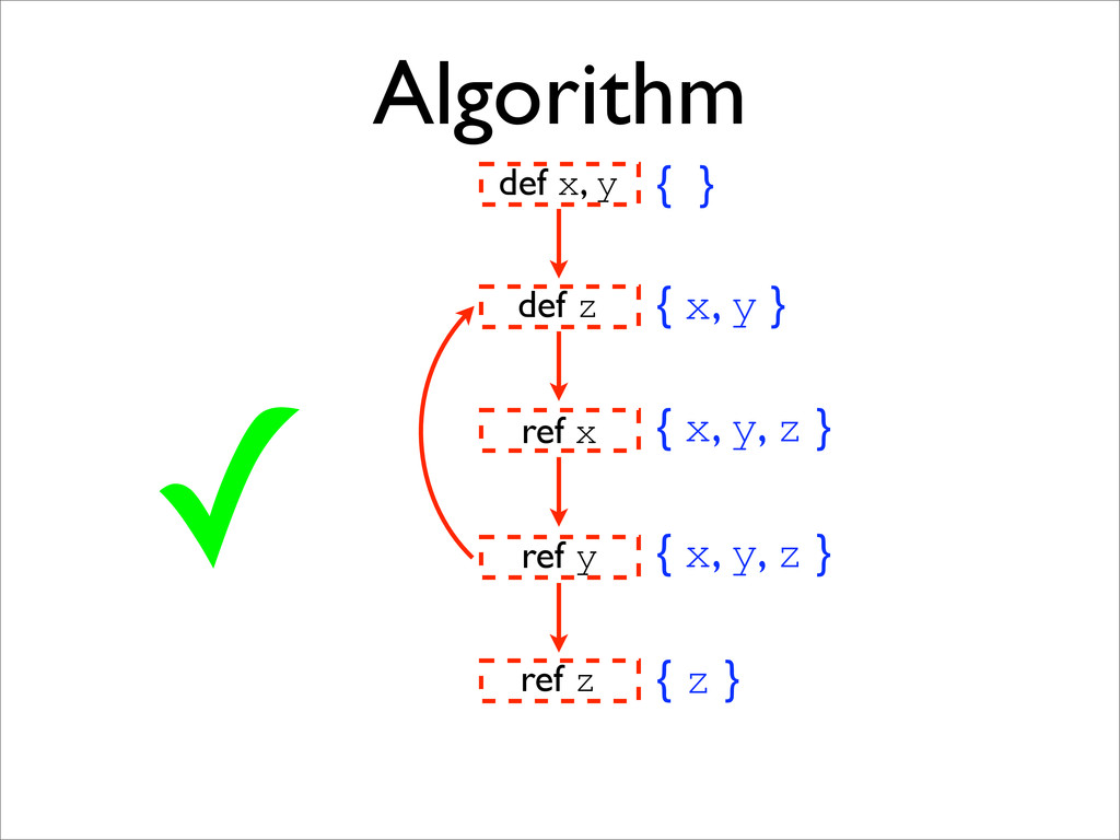
* A simple iterative algorithm can be used to find the smallest solution to the LVA data-flow equations
![Algorithm for i = 1 to n do live[i] :=](https://files.speakerdeck.com/presentations/4ea51e3b15006a0054007afc/slide_39.jpg)