Learning Noise in Quantum Information Processors

A talk I gave at the "Quantum Techniques in Machine Learning" workshop in Verona, Italy. Released under SAND2017-11820 C.

Transcript

1. Sandia National Laboratories is a multimission laboratory managed and operated by National Technology and Engineering Solutions of Sandia LLC, a wholly owned subsidiary of Honeywell International Inc. for the U.S. Department of Energy’s National Nuclear Security Administration under contract DE-NA0003525. CCR Center for Computing Research Learning Noise in Quantum Information Processors Travis L Scholten @Travis_Sch Center for Quantum Information and Control, University of New Mexico, Albuquerque, USA Center for Computing Research, Sandia National Laboratories, Albuquerque, USA QTML 2017
2. 3 quantum machine learning annealing quantum annealing quantum gibbs sampling quantum topological algorithms quantum rejection sampling / HHL Quantum ODE solvers control and metrology reinforcement learning tomography quantum control phase estimation hamiltonian learning quantum perceptron quantum BM simulated annealing markov chain monte-carlo neural nets feed forward neural net quantum PCA quantum SVM quantum NN classification quantum clustering quantum data fitting machine learning quantum information processing FIG. 1. Conceptual depiction of mutual crossovers between quantum and traditional machine learning. Biamonte, et. al, arXiv: 1611.09347 There are lots of applications at the intersection of QI/QC and ML… 26
3. 3 quantum machine learning annealing quantum annealing quantum gibbs sampling quantum topological algorithms quantum rejection sampling / HHL Quantum ODE solvers control and metrology reinforcement learning tomography quantum control phase estimation hamiltonian learning quantum perceptron quantum BM simulated annealing markov chain monte-carlo neural nets feed forward neural net quantum PCA quantum SVM quantum NN classification quantum clustering quantum data fitting machine learning quantum information processing FIG. 1. Conceptual depiction of mutual crossovers between quantum and traditional machine learning. Biamonte, et. al, arXiv: 1611.09347 …I want to focus on how ML can improve characterization of quantum hardware. 25
4. Quantum device characterization (QCVV) techniques arranged by amount learned and time required. Speed of learning Fast Full Slow Amount learned Limited 24
5. Tomography is very informative, but time-consuming! Gate set tomography State tomography Speed of learning Fast Slow Amount learned Process tomography Full Limited 23
6. Randomized benchmarking is fast, but yields limited information. Randomized Benchmarking Gate set tomography State tomography Speed of learning Fast Slow Amount learned Process tomography (Several variants, leads to different kinds of information learned.) Full Limited 22
7. Depending on how much we want to learn, and how quickly, machine learning could be useful. M achine Learning Randomized Benchmarking Gate set tomography State tomography Speed of learning Fast Slow Amount learned Process tomography Full Limited Caveat: “Speed” doesn’t include *training time* 21
8. Depending on how much we want to learn, and how quickly, machine learning could be useful. M achine Learning Randomized Benchmarking Gate set tomography State tomography Speed of learning Fast Slow Amount learned Process tomography Full Limited Can machine learning extract information about noise affecting near and medium-term quantum hardware? 20
9. Noise affects the outcome probabilities of quantum circuits. How can we learn about noise using the data we get from running quantum circuits? 19
10. suppose the reader would like to typeset the mple circuit: | 0 i Y⇡/2 typeset using C=1em @R=.7em { te{X} & \qw Noise in quantum hardware affects the outcome probabilities of circuits. (Noise affects outcome probability) 18 Example: over-rotation error of a single-qubit gate (The circuit we write down) Pr(0) = Tr(|0ih0|E(|0ih0|)) = 1 2 (1 sin ✓)
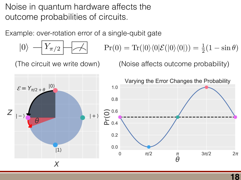
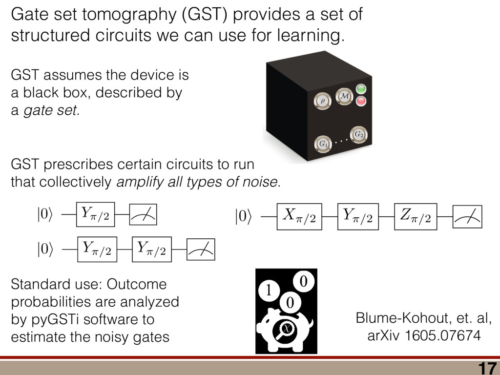
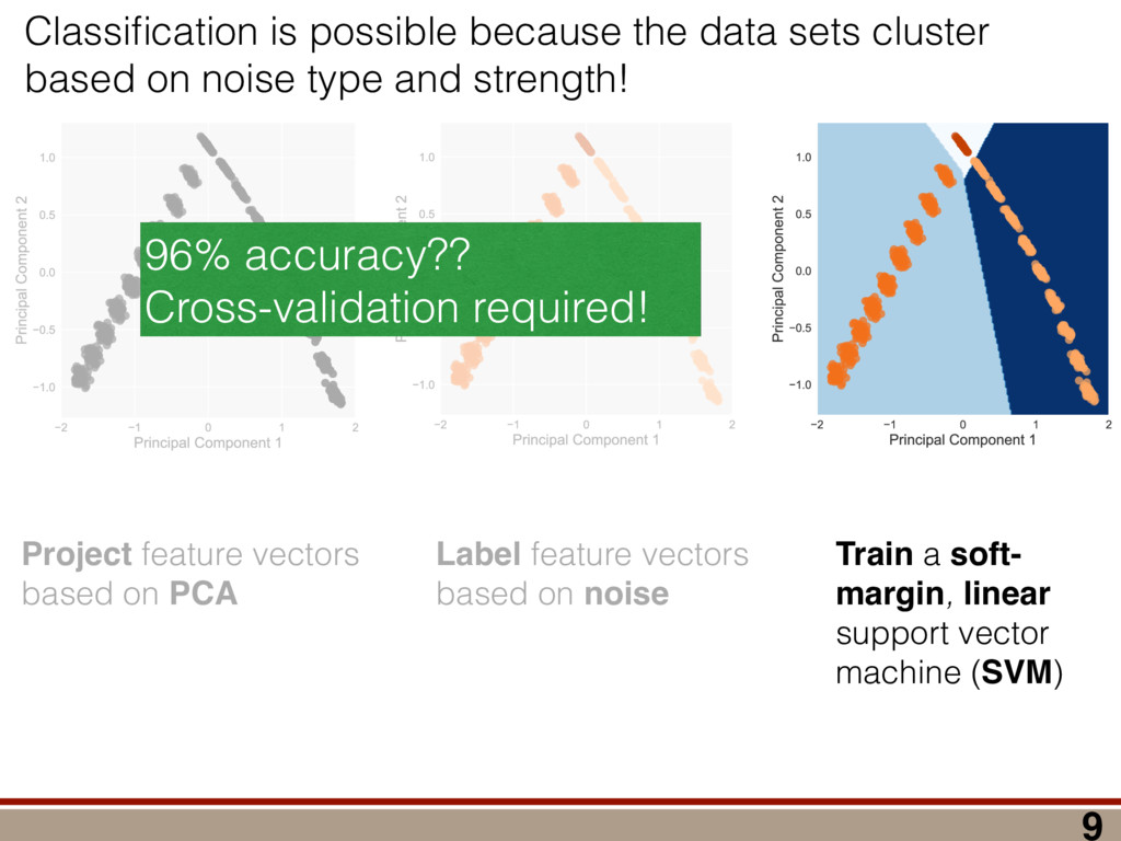
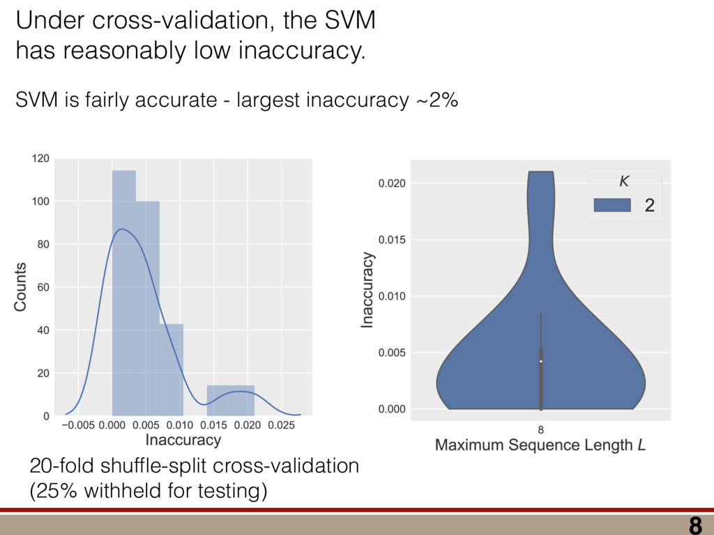
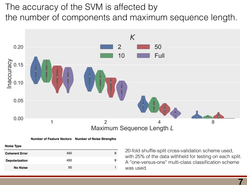
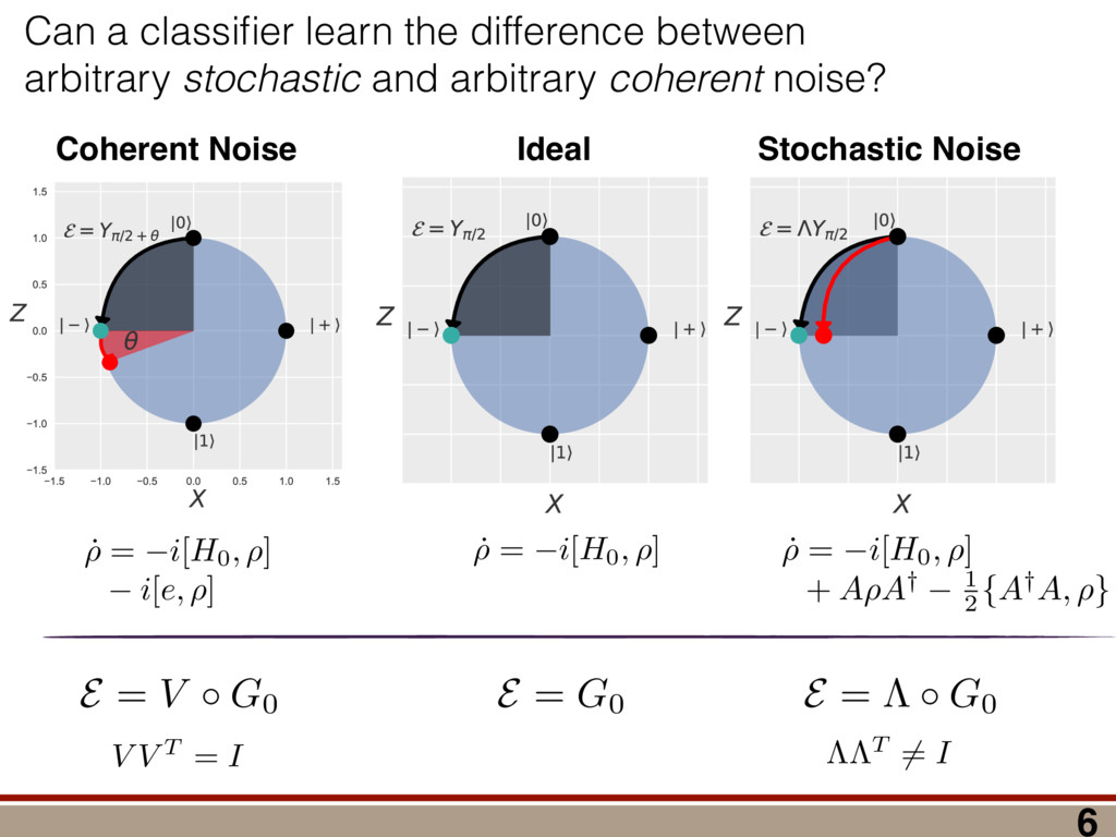
11. Gate set tomography (GST) provides a set of structured circuits we can use for learning. GST assumes the device is a black box, described by a gate set. GST prescribes certain circuits to run that collectively amplify all types of noise. Standard use: Outcome probabilities are analyzed by pyGSTi software to estimate the noisy gates (GST) for self-consistently characterizing an entire set of quantum logic gates on a black-box quan- tum device; (2) an explicit closed-form protocol for linear-inversion gate set tomography (LGST), whose reliability is independent of pathologies such as local maxima of the likelihood; and (3) a simple protocol for objectively scoring the accuracy of a tomographic estimate without reference to target gates, based on how well it predicts a set of testing experiments. We use gate set tomography to characterize a set of Cli↵ord-generating gates on a single trapped-ion qubit, and compare the performance of (i) standard process tomography; (ii) linear gate set tomography; and (iii) maximum likelihood gate set tomography. Quantum information processing (QIP) relies upon precise, repeatable quantum logic operations. Exper- iments in multiple QIP technologies [1–5] have imple- mented quantum logic gates with su cient precision to reveal weaknesses in the quantum tomography protocols used to characterize those gates. Conventional tomo- graphic methods assume and rely upon a precalibrated reference frame, comprising (1) the measurements per- formed on unknown states, and (2) for quantum process tomography, the test states that are prepared and fed into the process (gate) to be characterized. Standard process tomography on a gate G proceeds by repeating a series of experiments in which state ⇢ j is prepared and observable (a.k.a. POVM e↵ect) E k is observed, using the statistics of each such experiment to estimate the corresponding probability p k | j = Tr[E k G[⇢ j ]] (given by Born’s rule), and finally reconstructing G from many such probabilities. But, in most QIP technologies, the various test states (⇢ j ) and measurement outcomes (E k ) are not known ex- actly. Instead, they are implemented using the very same gates that process tomography is supposed to character- ize. The quantum device is e↵ectively a black box, ac- cessible only via classical control and classical outcomes of quantum measurements, and in this scenario standard tomography can be dangerously self-referential. If we do process tomography on gate G under the common assumption that the test states and measurement out- comes are both eigenstates of the Pauli x , y , z opera- tors, then the accuracy of the estimate ˆ G will be limited by the error in this assumption. This is now a critical experimental issue. In plat- forms including (but not limited to) superconducting flux qubits [1], trapped ions [5], and solid-state qubits, quan- tum logic gates are being implemented so precisely that systematic errors in tomography (due to miscalibrated reference frames) are glaringly obvious. Fixes have been proposed [1, 2, 6, 7], but none yet provide a general, comprehensive, reliable scheme for gate characterization. M ⇢ G1 G2 ... FIG. 1: The GST model of a quantum device. Gate set tomography treats the quantum system of interest as a black box, with strictly limited access. This is a fairly good model for many qubit technologies, especially those based on solid state and/or cryogenic technologies. We do not have direct access to the Hilbert space or any aspect of it. Instead, the device is controlled via buttons that implement various gates (including a preparation gate and a measurement that causes one of two indicator lights to illuminate). Prior information about the gates’ function may be available, and can be used, but should not be relied upon. In this article, we present gate set tomography (GST), a complete scheme for reliably and accurately charac- terizing an entire set of quantum gates. In particular we introduce the first linear-inversion protocol for self- consistent process tomography, linear gate set tomog- raphy (LGST). LGST is a closed-form estimation pro- tocol (inspired in part by [8–10]) that cannot – unlike pure maximum-likelihood (ML) algorithms – run afoul of local maxima in a likelihood function that is gener- Blume-Kohout, et. al, arXiv 1605.07674 } | A i \ bra { B } h B | { B } h A | B i \ op { A }{ B } | A ih B | { j }{ B }{ k } h j | B | k i \ expval { B } h B i SIMPLE QUANTUM CIRCUITS , suppose the reader would like to typeset the mple circuit: | 0 i Y⇡/2 typeset using @C=1em @R=.7em { ate{X} & \qw ive outputs: t { A } | A i \ bra { B } h B | { A }{ B } h A | B i \ op { A }{ B } | A ih B | em { j }{ B }{ k } h j | B | k i \ expval { B } h B i IV. SIMPLE QUANTUM CIRCUITS egin, suppose the reader would like to typeset the ng simple circuit: | 0 i Y⇡/2 Y⇡/2 was typeset using it @C=1em @R=.7em { \gate{X} & \qw grams using standard t and time consuming cro package designed wing quantum circuit an array. In a mat- asic syntax and start se qcircuit from the that they’ve learned the end of § IV, but ose that wish to type- the GNU public license. ndix C. \ ket { A } | A i \ bra { B } \ ip { A }{ B } h A | B i \ op { A }{ B } \ melem { j }{ B }{ k } h j | B | k i \ expval { B } IV. SIMPLE QUANTUM CIRCUIT To begin, suppose the reader would like to ty following simple circuit: | 0 i X⇡/2 Y⇡/2 Z⇡/2 This was typeset using \Qcircuit @C=1em @R=.7em { & \gate{X} & \qw } 17
12. ucting an array. In a mat- the basic syntax and start n. to use qcircuit from the find that they’ve learned w by the end of § IV, but or those that wish to type- under the GNU public license. Appendix C. IV. SIMPLE QUANTUM CIRCUIT To begin, suppose the reader would like to typ following simple circuit: | 0 i Y⇡/2 Y⇡/2 Y⇡/2 Y⇡/2 This was typeset using \Qcircuit @C=1em @R=.7em { & \gate{X} & \qw } Gate set tomography (GST) provides a set of structured circuits we can use for learning. GST prescribes certain circuits to run that collectively amplify all types of noise. IMPLE QUANTUM CIRCUITS ppose the reader would like to typeset the le circuit: | 0 i Y⇡/2 peset using 1em @R=.7em { {X} & \qw { j }{ B }{ k } h j | B | k i \ expval { B } h B i SIMPLE QUANTUM CIRCUITS n, suppose the reader would like to typeset the imple circuit: | 0 i Y⇡/2 Y⇡/2 s typeset using @C=1em @R=.7em { ate{X} & \qw Circuits have varying length, up to some maximum length L. l = 1, 2, 4, · · · , L l = 1 l = 2 Why? Longer circuits are more sensitive to noise. 16 l = 4 l = 1 l = 2
13. To do machine learning on GST data sets, embed them in a feature space. ## Columns = minus count, plus count {} 100 0 Gx 44 56 Gy 45 55 GxGx 9 91 GxGxGx 68 32 GyGyGy 70 30 (GST data set) f = (f1, f2, · · · ) 2 Rd The dimension of the feature space grows with L because more circuits are added. 0 B B B B B B @ 0 .56 .55 .91 .32 .3 1 C C C C C C A 15
14. Noise changes some components of the feature vectors. How can we identify the “signature” of a noise process using GST feature vectors? 14
15. Principal component analysis (PCA) is a useful tool for understanding the structure of GST feature vectors. PCA finds a low-dimensional representation of data by looking for directions of maximum variance. Compute covariance matrix & diagonalize Defines a map: f ! PK j=1 (f · j) j C = PK j=1 j j T j 1 2 · · · K (d = K) 13
16. Projection onto a 2-dimensional PCA subspace reveals a structure to GST feature vectors. Different noise types and noise strengths tend to cluster! (PCA performed on entire dataset, then individual feature vectors transformed.) 4.5% depolarizing 1% coherent 1% depolarizing 4.5% coherent 12
17. Longer GST circuits amplify noise, making the clusters more distinguishable. Adding longer circuits makes the clusters more distinguishable. We can use this structure to do classification! (An independent PCA was done for each L.) 11
18. Classification is possible because the data sets cluster based on noise type and strength! Project feature vectors based on PCA 10 Label feature vectors based on noise Train a soft- margin, linear support vector machine (SVM)
19. Classification is possible because the data sets cluster based on noise type and strength! Project feature vectors based on PCA 9 Label feature vectors based on noise Train a soft- margin, linear support vector machine (SVM) 96% accuracy?? Cross-validation required!
20. Under cross-validation, the SVM has reasonably low inaccuracy. 8 SVM is fairly accurate - largest inaccuracy ~2% 20-fold shuffle-split cross-validation (25% withheld for testing)
21. 7 20-fold shuffle-split cross-validation scheme used, with 25% of the data withheld for testing on each split. A “one-versus-one” multi-class classification scheme was used. The accuracy of the SVM is affected by the number of components and maximum sequence length.
22. Can a classifier learn the difference between arbitrary stochastic and arbitrary coherent noise? 6 Coherent Noise Ideal Stochastic Noise ˙ ⇢ = i[H0 , ⇢] ˙ ⇢ = i[H0 , ⇢] + A⇢A† 1 2 {A†A, ⇢} ˙ ⇢ = i[H0 , ⇢] i[e, ⇢] E = ⇤ G0 E = V G0 E = G0 V V T = I ⇤⇤T 6= I
23. Classification in a 2-dimensional subspace is harder, due to structure of PCA-projected feature vectors. 5 “Radio dish” type structure Linear classifier infeasible with only 2 PCA components
24. Preliminary results indicate a linear, soft-margin SVM can classify these two noise types in higher dimensions. 4 20-fold shuffle-split cross-validation scheme used, with 25% of the data withheld for testing on each split. A “one-verus-one” multi-class classification scheme was used. For each L: - 10 values of noise strength in [10**-4, 10**-1] - 260 random instances Gap goes away if noise <= 10**-2 removed from data
25. M achine Learning Specific machine learning tools can analyze GST circuits and learn about noise. Randomized Benchmarking Gate set tomography State tomography Speed of learning Fast Slow Amount learned Process tomography Full Limited SVMs & PCA + GST Circuits 3
26. M achine Learning Randomized Benchmarking Gate set tomography State tomography Speed of learning Fast Slow Amount learned Process tomography Full Limited What else can we learn?? What circuits do we need?? SVMs & PCA + GST Circuits 2 Specific machine learning tools can analyze GST circuits and learn about noise.
27. 3 quantum machine learning annealing quantum annealing quantum gibbs sampling quantum topological algorithms quantum rejection sampling / HHL Quantum ODE solvers control and metrology reinforcement learning tomography quantum control phase estimation hamiltonian learning quantum perceptron quantum BM simulated annealing markov chain monte-carlo neural nets feed forward neural net quantum PCA quantum SVM quantum NN classification quantum clustering quantum data fitting machine learning quantum information processing FIG. 1. Conceptual depiction of mutual crossovers between quantum and traditional machine learning. b. Controlling quantum systems Learning methods have also seen ample success in developing in the development of quantum computation and infor- mation science) [34–37]. In the presence of noise and Biamonte, et. al, arXiv: 1611.09347 1 There are lots of problems at the intersection of device characterization and machine learning!
28. Thank you! @Travis_Sch 0