Georgia Tech Intern

Transcript

1. A Fast Multipole Method for the Rotne-Proger-Yamakawa tensor for Polydisperse Particle Systems Vipul Harsh India 8thMay, 2014 Vipul Harsh (India) Georgia Tech. Symposium 8thMay, 2014 1 / 22
2. Outline 1 Introduction 2 Contribution 3 Barnes Hut 4 Barnes Hut Algorithm : Basic Idea 5 Fast Multipole Method 6 RPY tensor 7 Existing Work 8 Kernel Independent FMM 9 Brownian Dynamics 10 Timings 11 Conclusion Vipul Harsh (India) Georgia Tech. Symposium 8thMay, 2014 2 / 22
3. Introduction Introduction Why do we need better and faster algorithms? The naive algorithm is of quadratic complexity. The algorithm doesn’t even scale for as less as 105 particles. Speed is achieved at the expense of accuracy. There are different algorithms to solve the problem approximately. Vipul Harsh (India) Georgia Tech. Symposium 8thMay, 2014 3 / 22
4. Contribution Contribution RPY tensor has already been done for same sized particles. However, most biological and physical systems comprise of different sized particles, for instance molecules within a cell are of different sizes. We have done multiple sized particles, which is new using state of the art methods. We also exploit threading and use multiple cores for the computation. The timings we are getting is very promising. We are able to do 106 particles within 2 minutes. This could help simulate large systems which has several biological and physical applications. Vipul Harsh (India) Georgia Tech. Symposium 8thMay, 2014 4 / 22
5. Barnes Hut Barnes Hut Algorithm : Basic Idea A collection of particles far away from a single particle influence it in similar ways. The collection of particles can be approximated by a large point particle and the force(or potential) may be computed using that particle. We employ this technique very often without even realizing it. For instance, we don’t see the sun as a huge collection of particles(which infact, it is). Instead, we treat the sun as a single large particle and use it’s center to compute the gravitational force exerted by the sun on say, the Earth. Vipul Harsh (India) Georgia Tech. Symposium 8thMay, 2014 5 / 22
6. Fast Multipole Method Fast Multipole Method: Basic Idea We are interested in computing sums of the form. f(xk ) = N n=1,n=k K(xk , xn )q(xn ) Suppose that, the Kernel function K is degenerate, i.e. K(x, y) = p i=1 φi (x) ψi (y) Then, f(xk ) becomes, f(xk ) = N n=1,n=k p i=1 φi (xk )ψi (xn )q(xn ) = p i=1 N n=1,n=k ψi (xn )q(xn ) φi (xk ) (1) Vipul Harsh (India) Georgia Tech. Symposium 8thMay, 2014 6 / 22
7. Fast Multipole Method Fast Multipole Method: Basic Idea, Continued We can compute these p sums beforehand. So overall, the final algorithm can be performed in O(pN) time. In practice, the Kernel function is rarely degenerate. Instead we expand the Kernel function into an infinite converging series, and then take the first p terms. K(x, y) = ∞ i=1 ψi (x)φi (y) ≈ p i=1 ψi (x)φi (y) (2) Vipul Harsh (India) Georgia Tech. Symposium 8thMay, 2014 7 / 22
8. RPY tensor RPY tensor for same sized particles For equal sized particles, the RPY tensor D(x,y) is the following : D(x, y) =      kβ T 8πη [(1 r I + r⊗r r3 ) + 2a2 3r3 (1 − 3r⊗r r2 )] r ≥ 2a kβ T 6πηa [(1 − 9r 32a )I + 3 32a r⊗r r ] r < 2a Vipul Harsh (India) Georgia Tech. Symposium 8thMay, 2014 8 / 22
9. RPY tensor RPY tensor for different sized particles For different sized particles, the radius in the RPY tensor is replaced by effective radius. D(x, y) =      kβ T 8πη [(1 r I + r⊗r r3 ) + (a2 x +a2 y ) 3r3 (1 − 3r⊗r r2 )] r ≥ ax + ay kβ T 6πηa [(1 − 9r 32a )I + 3 32a r⊗r r ] r < ax + ay Where a = effective radius = (a2 x +a2 y ) 2 Vipul Harsh (India) Georgia Tech. Symposium 8thMay, 2014 9 / 22
10. Existing Work Existing Work We’re interested in computing the following sum, um i = n i=1 3 j=1 Dij (xm, xn)vn j The classical FMM for coulombic interactions is as follows. Pm(q, p, d) = N n=1,n=m qn rmn + N n=1,n=m (dn.rmn )pn r3 mn Fi m (q, p, d) = δPm(q, p, d) δxm i Vipul Harsh (India) Georgia Tech. Symposium 8thMay, 2014 10 / 22
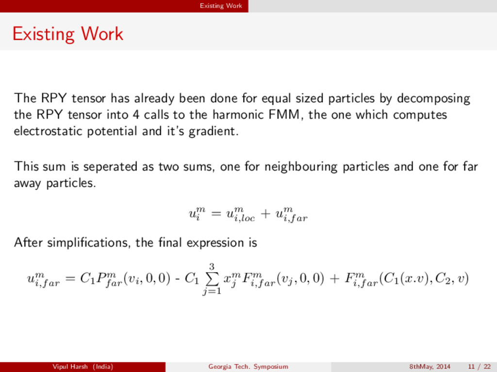
11. Existing Work Existing Work The RPY tensor has already been done for equal sized particles by decomposing the RPY tensor into 4 calls to the harmonic FMM, the one which computes electrostatic potential and it’s gradient. This sum is seperated as two sums, one for neighbouring particles and one for far away particles. um i = um i,loc + um i,far After simplifications, the final expression is um i,far = C1 Pm far (vi , 0, 0) - C1 3 j=1 xm j Fm i,far (vj , 0, 0) + Fm i,far (C1 (x.v), C2 , v) Vipul Harsh (India) Georgia Tech. Symposium 8thMay, 2014 11 / 22
12. Existing Work RPY tensor for different sized particles For different sized particles, the sum can be computed using 5 calls to the Harmonic FMM routine. um i,far = C1 Pm far (vi , 0, 0) − C1 3 j=1 xm j Fm i,far (vj , 0, 0)+ Fm i,far (C1 (x.v), C2 , a2 n 2 .v) + a2 m 2 Fm i,far (0, C2 , v) (3) Vipul Harsh (India) Georgia Tech. Symposium 8thMay, 2014 12 / 22
13. Kernel Independent FMM Kernel Independent FMM Recently there have been attempts to generalize the FMM for any Kernel function that smoothens for large r. These aim at computing sums of the form, f(xi ) = N j=1 K(xi , yj )q(yj ) Where, y1 ,...yN are the ”source” points and x1 ,...xN are the ”target” points at which the potential needs to be computed. In our case, the target points are the same as source points. Vipul Harsh (India) Georgia Tech. Symposium 8thMay, 2014 13 / 22
14. Kernel Independent FMM Kernel Independent FMM We implemented the RPY tensor for different sized particles using KIFMM with 2 calls to the KIFMM. um i = N n=1 3 n=1 Dij (xm, xn)vn j = n i=1 3 j=1 kβ T 8πη [(1 r I + r⊗r r3 ) + (a2 m +a2 n ) 3r3 (1 − 3r⊗r r2 )]ij vn j = n i=1 3 j=1 kβ T 8πη [(1 r I + r⊗r r3 ) + a2 n 3r3 (1 − 3r⊗r r2 )]ij vn j +a2 m n i=1 3 j=1 kβ T 8πη [ 1 3r3 (1 − 3r⊗r r2 )]ij vn j Vipul Harsh (India) Georgia Tech. Symposium 8thMay, 2014 14 / 22
15. Brownian Dynamics Adding Brownian dynamics Brownian forces for each particles is a (N × 3) multivariate gaussian distribution with the entries of the covariance matrix being the corresponding RPY tensor. To generate such a distribution, we generate a standard normal (N × 3) multivariate gaussian distribution. Multiplying this distribution with the square root of the covariance matrix gives a vector with the required distribution. However, it is expensive to compute the square root directly. Instead we use an approximation to the square root. √ Dz ≈ T i=1 ai Diz Dz can be computed using FMM, and hence is not computationally expensive. This way, we avoid computing √ D explicitly. Vipul Harsh (India) Georgia Tech. Symposium 8thMay, 2014 15 / 22
16. Timings Monodisperse vs Polydisperse There’s just one call to the KIFMM routine for Monodisperse particles (as opposed to two calls for polydisperse particles). Thus, we expect the KIFMM method to take twice as much time for polydisperse particles. For the 5 call method, there are 5 calls instead of 4. The extra call has dipole moments and hence should take a little more than a call without dipole moments. Vipul Harsh (India) Georgia Tech. Symposium 8thMay, 2014 16 / 22
17. Timings Timings nparticles KIFMM 5 call FMM Naive 100 2170 5 2 300 2174 17 25 600 2220 55 130 1000 2289 142 374 3000 4287 744 4288 5000 5309 1734 13469 10000 8029 4270 53083 Table 1 : Comparison of computation times.Time units - ms Vipul Harsh (India) Georgia Tech. Symposium 8thMay, 2014 17 / 22
18. Timings Timings nparticles KIFMM 5 call FMM Naive 15000 10179 6216 - 20000 12667 8568 - 25000 15887 8745 - 30000 26993 11034 - 35000 34050 13915 - 40000 41125 24857 - 45000 44161 37953 - 50000 45639 33962 - 100000 68151 41671 - Table 2 : Comparison of computation times. Time units - ms Vipul Harsh (India) Georgia Tech. Symposium 8thMay, 2014 18 / 22
19. Timings Parallel KIFMM Timings Cores PKIFMM(sec) SpeedUp 1 642 1 2 354 1.81 4 191 3.36 6 145 4.43 8 124 5.18 10 106 6.06 12 111 5.78 16 113 5.68 20 110 5.84 24 127 5.06 Table 3 : Computation times with multiple cores for 106 particles Vipul Harsh (India) Georgia Tech. Symposium 8thMay, 2014 19 / 22
20. Timings Timings Comparison Vipul Harsh (India) Georgia Tech. Symposium 8thMay, 2014 20 / 22
21. Conclusion Conclusion We have presented two fast methods for doing large scale simulations for polydisperse particle systems involving hydrodynamic interactions and RPY tensor. We have extended the 4 call method for polydisperse particle systems, which involves 5 calls to the harmonic FMM. We have used the parallel version of the Kernel Independent FMM to run the simulations. We ran our experiments with multiple cores and achieved a decent speedup. Vipul Harsh (India) Georgia Tech. Symposium 8thMay, 2014 21 / 22
22. Conclusion Thank you! Vipul Harsh (India) Georgia Tech. Symposium 8thMay, 2014 22 / 22