Dynamic Tree Problem Self Adjusting Binary Search Tree (D. Sleator, R. Tarjan, 1985) Jongwook Choi and Taihyun Hwang Seoul National University 4541.561 Advanced Computation Theory Term Project June 7, 2011
Splay Tree is a simple BST with Splay operation. The Splay operation is a kind of restructuring heuristic, applying tree rotations to move the last-accessed node to the root. Due to the Splay operation, costs of operations are reduced to O (log n ) . Furthermore, it performs especially well on special access patterns.
following, T, T0 are splay trees and x are nodes. Splay( T, x ) move the node x of T to the root. Find( T, k ) find the node x with key k. Insert( T, k ) insert a new node with key k into T. Delete( T, x ) delete the node x of T.
following, T, T0 are splay trees and x are nodes. Splay( T, x ) move the node x of T to the root. Find( T, k ) find the node x with key k. Insert( T, k ) insert a new node with key k into T. Delete( T, x ) delete the node x of T. Split( T, k ) Join( T 1 , T 2) . . . All the cost of above operations are O (log n ) amortized, O ( n ) worst.
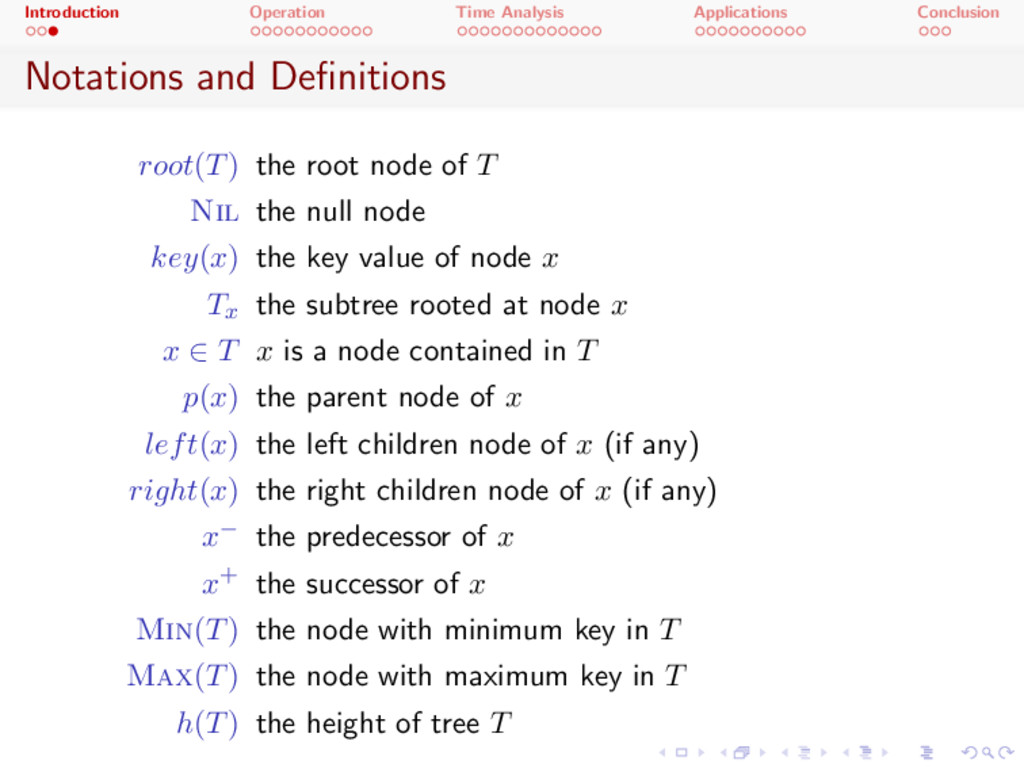
( T ) the root node of T Nil the null node key ( x ) the key value of node x Tx the subtree rooted at node x x 2 T x is a node contained in T p ( x ) the parent node of x left ( x ) the left children node of x (if any) right ( x ) the right children node of x (if any) x the predecessor of x x+ the successor of x Min( T ) the node with minimum key in T Max( T ) the node with maximum key in T h ( T ) the height of tree T
T, x ) : moves the node x to the root of T. If x = root ( T ) , nothing to do. We will denote x’s parent by y and x’s grandparent by z. Figure: Splay (T, a)
Step (Zig-zig) : if x and y are either both left or both right childrens 1 Let z be the parent of y. 2 Rotate the edge ( y, z ) , making y a root. 3 Rotate the edge ( x, y ) , making x a root. Figure: Zig-zig
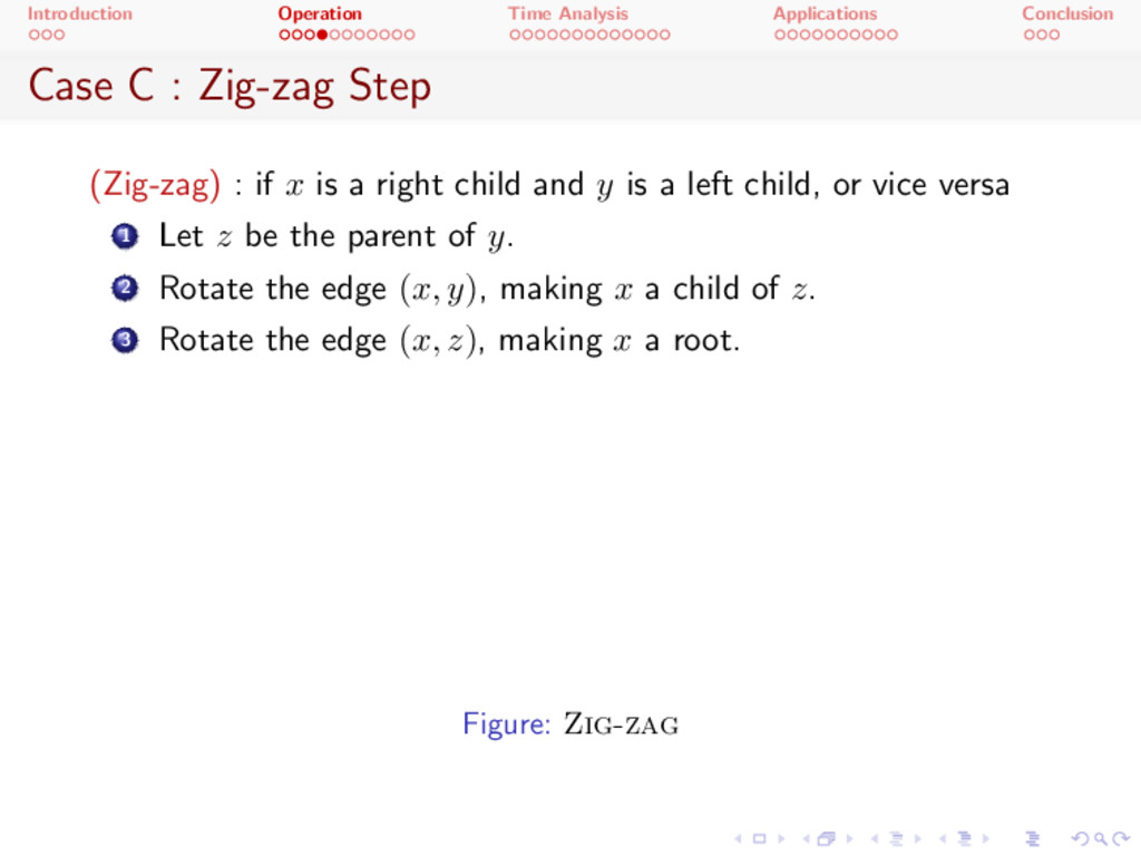
Step (Zig-zag) : if x is a right child and y is a left child, or vice versa 1 Let z be the parent of y. 2 Rotate the edge ( x, y ) , making x a child of z. 3 Rotate the edge ( x, z ) , making x a root. Figure: Zig-zag
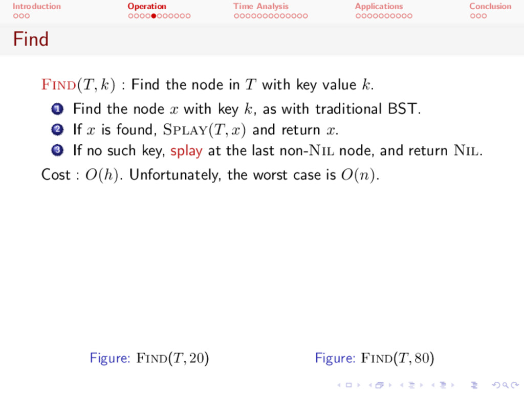
) : Find the node in T with key value k. 1 Find the node x with key k, as with traditional BST. 2 If x is found, Splay( T, x ) and return x. 3 If no such key, splay at the last non- Nil node, and return Nil . Cost : O ( h ) . Unfortunately, the worst case is O ( n ) . Figure: Find (T, 20 ) Figure: Find (T, 80 )
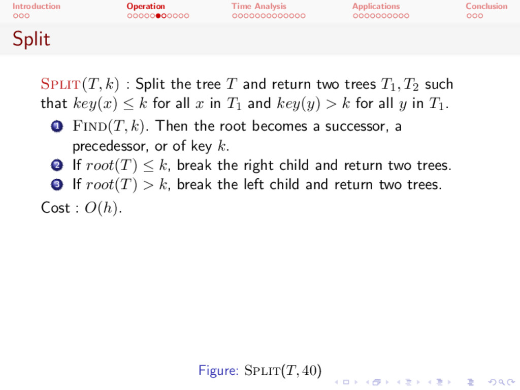
) : Split the tree T and return two trees T 1 , T 2 such that key ( x ) k for all x in T 1 and key ( y ) > k for all y in T 1 . 1 Find( T, k ) . Then the root becomes a successor, a precedessor, or of key k. 2 If root ( T ) k, break the right child and return two trees. 3 If root ( T ) > k, break the left child and return two trees. Cost : O ( h ) . Figure: Split (T, 40 )
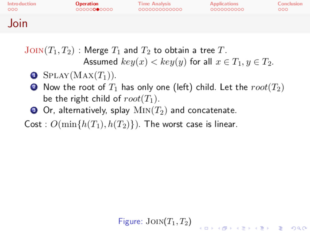
, T 2) : Merge T 1 and T 2 to obtain a tree T. Assumed key ( x ) < key ( y ) for all x 2 T 1 , y 2 T 2 . 1 Splay(Max( T 1)) . 2 Now the root of T 1 has only one (left) child. Let the root ( T 2) be the right child of root ( T 1) . 3 Or, alternatively, splay Min( T 2) and concatenate. Cost : O (min {h ( T 1) , h ( T 2) } ) . The worst case is linear. Figure: Join (T1 , T2 )
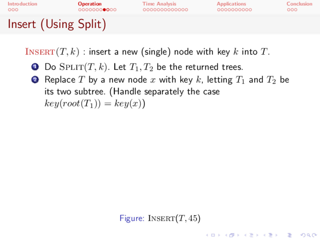
T, k ) : insert a new (single) node with key k into T. 1 Do Split( T, k ) . Let T 1 , T 2 be the returned trees. 2 Replace T by a new node x with key k, letting T 1 and T 2 be its two subtree. (Handle separately the case key ( root ( T 1)) = key ( x ) ) Figure: Insert (T, 45 )
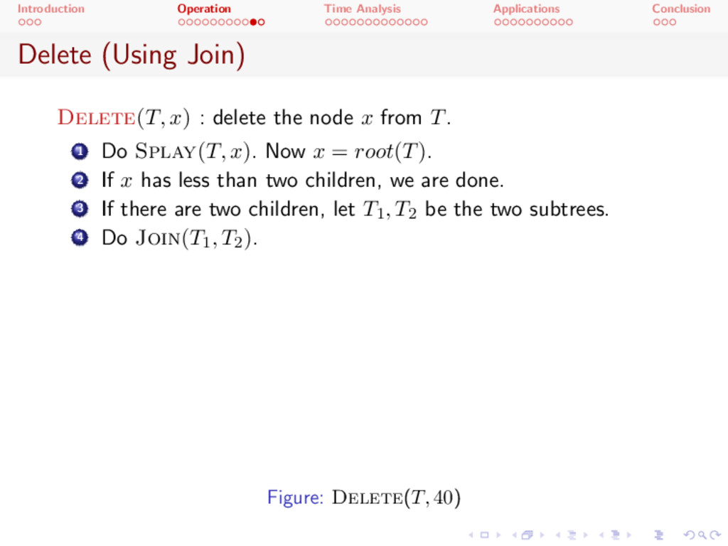
T, x ) : delete the node x from T. 1 Do Splay( T, x ) . Now x = root ( T ) . 2 If x has less than two children, we are done. 3 If there are two children, let T 1 , T 2 be the two subtrees. 4 Do Join( T 1 , T 2) . Figure: Delete (T, 40 )
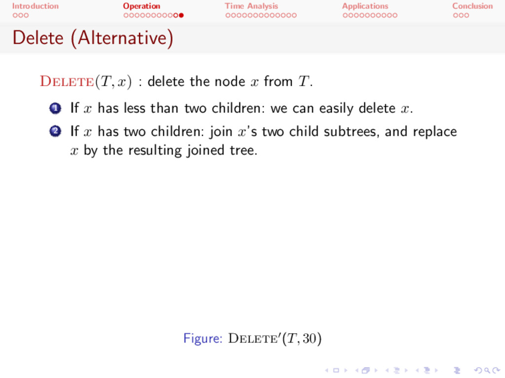
x ) : delete the node x from T. 1 If x has less than two children: we can easily delete x. 2 If x has two children: join x’s two child subtrees, and replace x by the resulting joined tree. Figure: Delete 0(T, 30 )
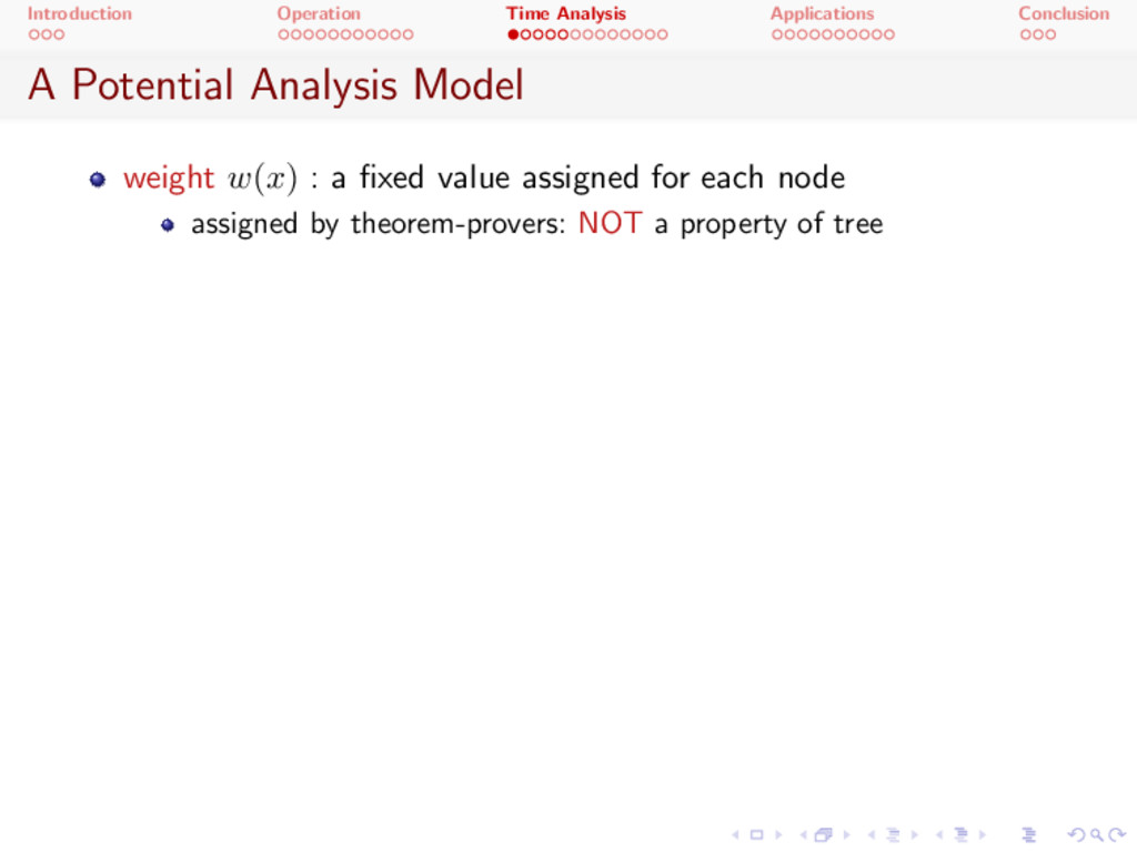
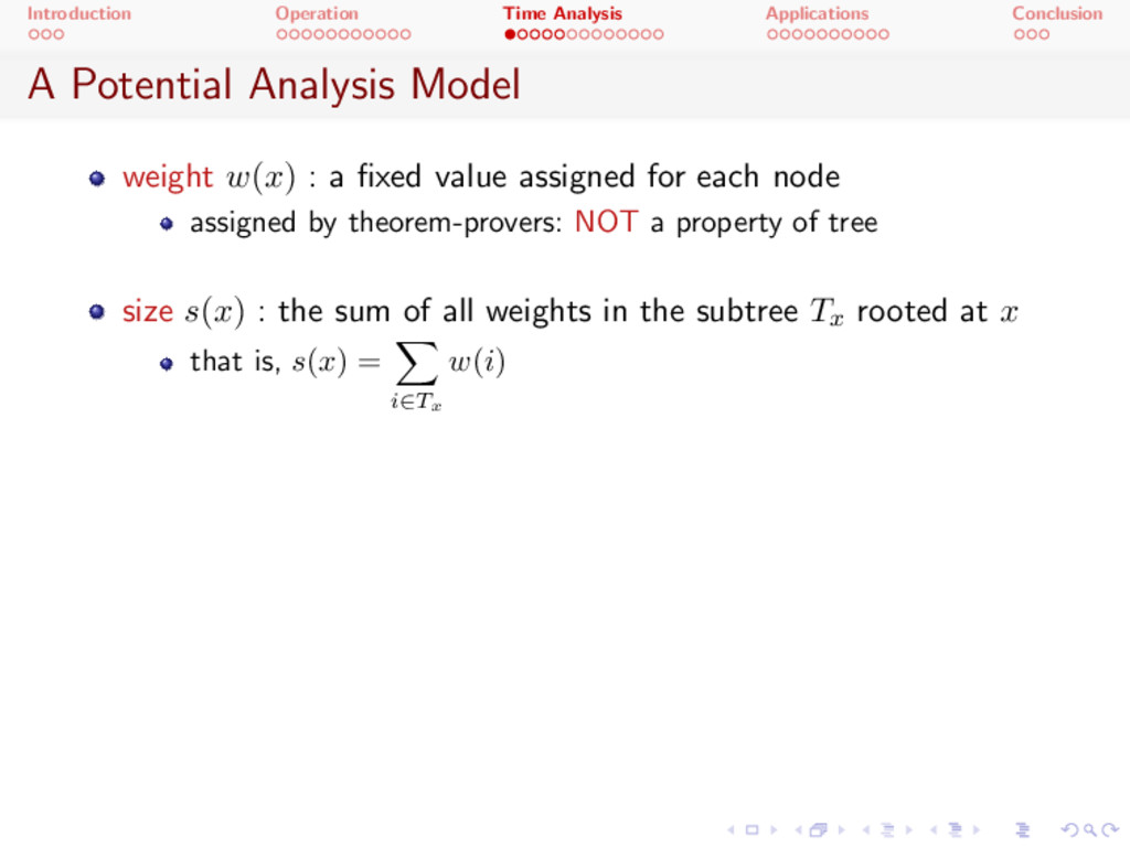
weight w ( x ) : a fixed value assigned for each node assigned by theorem-provers: NOT a property of tree size s ( x ) : the sum of all weights in the subtree Tx rooted at x that is, s ( x ) = X i 2 Tx w ( i )
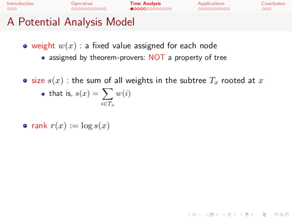
weight w ( x ) : a fixed value assigned for each node assigned by theorem-provers: NOT a property of tree size s ( x ) : the sum of all weights in the subtree Tx rooted at x that is, s ( x ) = X i 2 Tx w ( i ) rank r ( x ) := log s ( x )
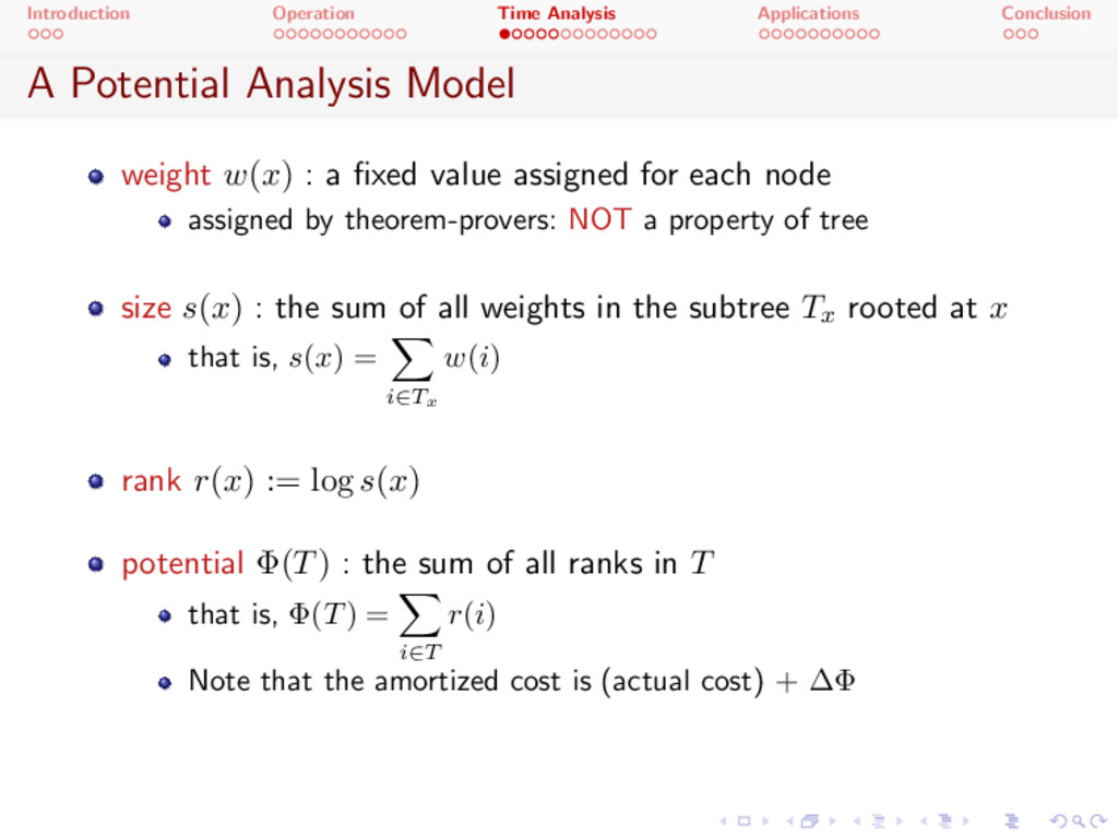
weight w ( x ) : a fixed value assigned for each node assigned by theorem-provers: NOT a property of tree size s ( x ) : the sum of all weights in the subtree Tx rooted at x that is, s ( x ) = X i 2 Tx w ( i ) rank r ( x ) := log s ( x ) potential ( T ) : the sum of all ranks in T that is, ( T ) = X i 2 T r ( i ) Note that the amortized cost is (actual cost) +
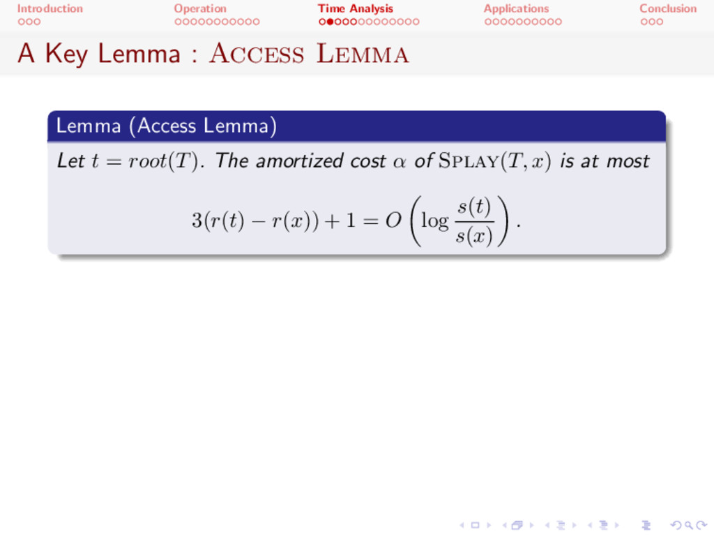
Access Lemma Lemma (Access Lemma) Let t = root ( T ) . The amortized cost ↵ of Splay( T, x ) is at most 3( r ( t ) r ( x )) + 1 = O ✓ log s ( t ) s ( x ) ◆ .
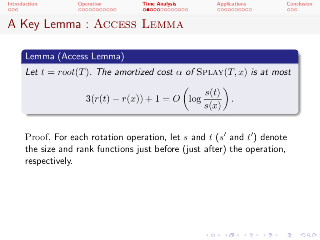
Access Lemma Lemma (Access Lemma) Let t = root ( T ) . The amortized cost ↵ of Splay( T, x ) is at most 3( r ( t ) r ( x )) + 1 = O ✓ log s ( t ) s ( x ) ◆ . Proof . For each rotation operation, let s and t (s0 and t0) denote the size and rank functions just before (just after) the operation, respectively.
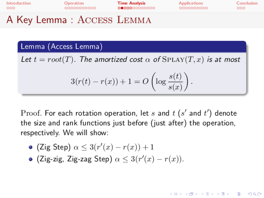
Access Lemma Lemma (Access Lemma) Let t = root ( T ) . The amortized cost ↵ of Splay( T, x ) is at most 3( r ( t ) r ( x )) + 1 = O ✓ log s ( t ) s ( x ) ◆ . Proof . For each rotation operation, let s and t (s0 and t0) denote the size and rank functions just before (just after) the operation, respectively. We will show: (Zig Step) ↵ 3( r0 ( x ) r ( x )) + 1 (Zig-zig, Zig-zag Step) ↵ 3( r0 ( x ) r ( x )) .
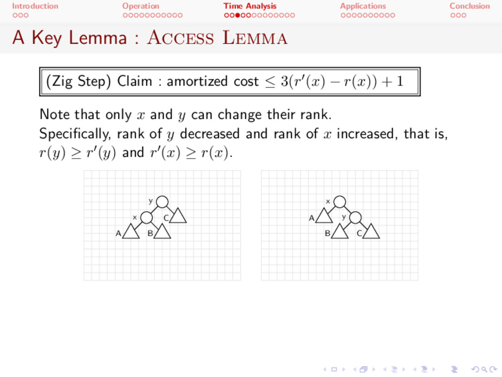
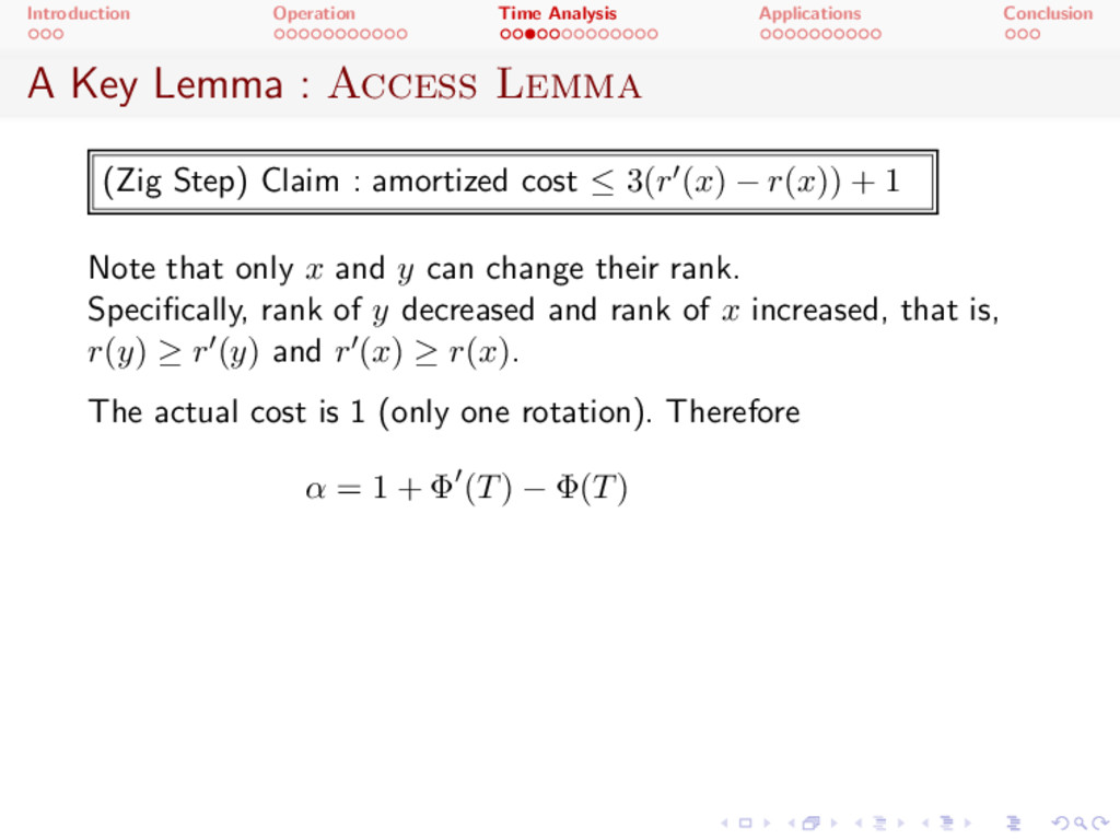
Access Lemma (Zig Step) Claim : amortized cost 3( r0 ( x ) r ( x )) + 1 Note that only x and y can change their rank. Specifically, rank of y decreased and rank of x increased, that is, r ( y ) r0 ( y ) and r0 ( x ) r ( x ) . x y A B C x y A B C
Access Lemma (Zig Step) Claim : amortized cost 3( r0 ( x ) r ( x )) + 1 Note that only x and y can change their rank. Specifically, rank of y decreased and rank of x increased, that is, r ( y ) r0 ( y ) and r0 ( x ) r ( x ) . The actual cost is 1 (only one rotation). Therefore ↵ = 1 + 0 ( T ) ( T )
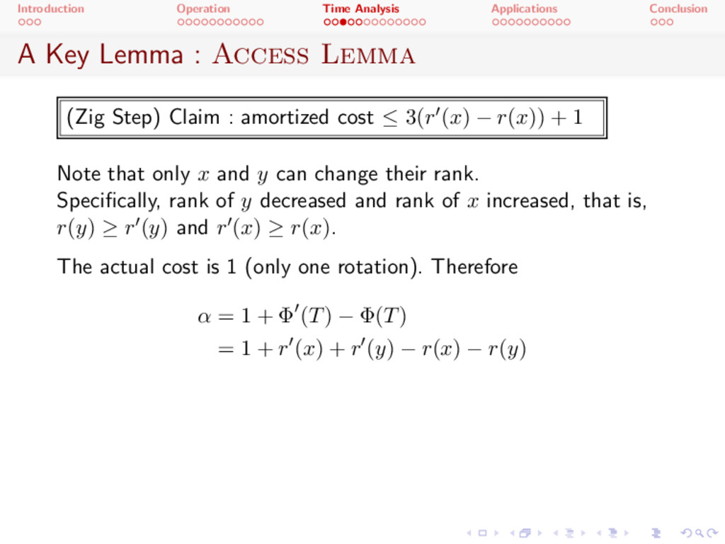
Access Lemma (Zig Step) Claim : amortized cost 3( r0 ( x ) r ( x )) + 1 Note that only x and y can change their rank. Specifically, rank of y decreased and rank of x increased, that is, r ( y ) r0 ( y ) and r0 ( x ) r ( x ) . The actual cost is 1 (only one rotation). Therefore ↵ = 1 + 0 ( T ) ( T ) = 1 + r0 ( x ) + r0 ( y ) r ( x ) r ( y )
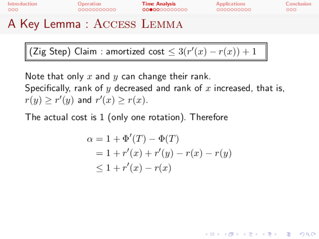
Access Lemma (Zig Step) Claim : amortized cost 3( r0 ( x ) r ( x )) + 1 Note that only x and y can change their rank. Specifically, rank of y decreased and rank of x increased, that is, r ( y ) r0 ( y ) and r0 ( x ) r ( x ) . The actual cost is 1 (only one rotation). Therefore ↵ = 1 + 0 ( T ) ( T ) = 1 + r0 ( x ) + r0 ( y ) r ( x ) r ( y ) 1 + r0 ( x ) r ( x )
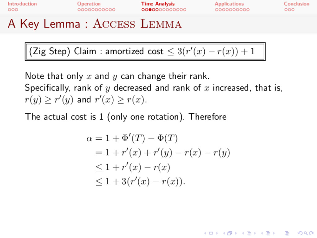
Access Lemma (Zig Step) Claim : amortized cost 3( r0 ( x ) r ( x )) + 1 Note that only x and y can change their rank. Specifically, rank of y decreased and rank of x increased, that is, r ( y ) r0 ( y ) and r0 ( x ) r ( x ) . The actual cost is 1 (only one rotation). Therefore ↵ = 1 + 0 ( T ) ( T ) = 1 + r0 ( x ) + r0 ( y ) r ( x ) r ( y ) 1 + r0 ( x ) r ( x ) 1 + 3( r0 ( x ) r ( x )) .
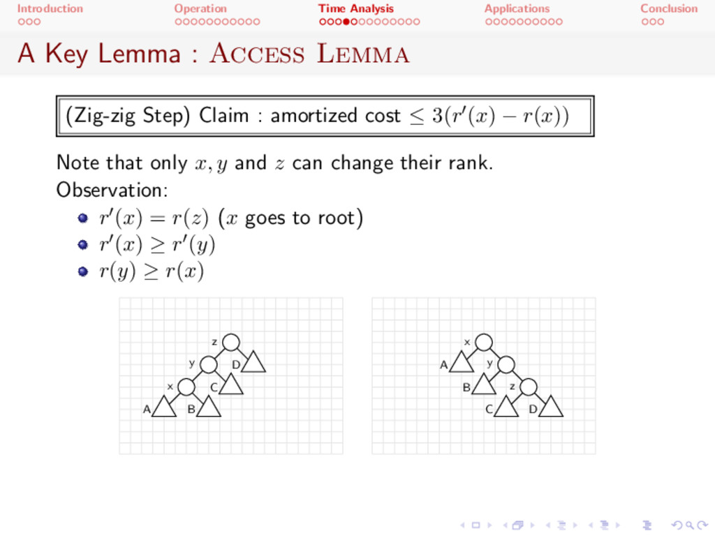
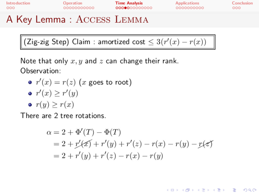
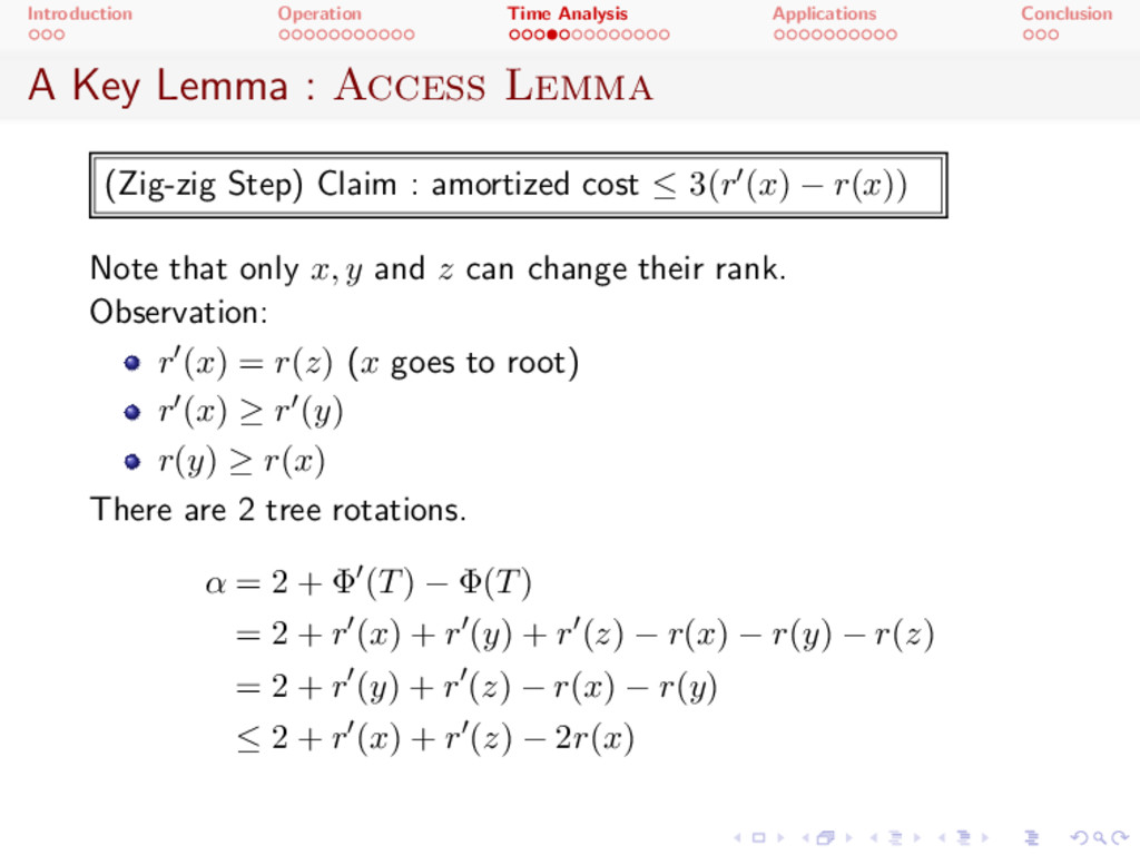
Access Lemma (Zig-zig Step) Claim : amortized cost 3( r0 ( x ) r ( x )) Note that only x, y and z can change their rank. Observation: r0 ( x ) = r ( z ) (x goes to root) r0 ( x ) r0 ( y ) r ( y ) r ( x ) x y z A B C D x y z A B C D
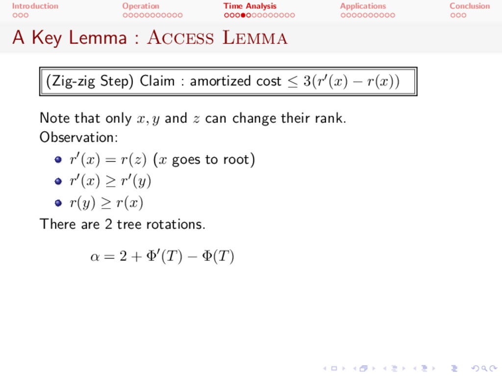
Access Lemma (Zig-zig Step) Claim : amortized cost 3( r0 ( x ) r ( x )) Note that only x, y and z can change their rank. Observation: r0 ( x ) = r ( z ) (x goes to root) r0 ( x ) r0 ( y ) r ( y ) r ( x ) There are 2 tree rotations. ↵ = 2 + 0 ( T ) ( T )
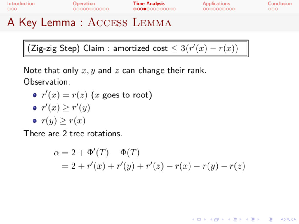
Access Lemma (Zig-zig Step) Claim : amortized cost 3( r0 ( x ) r ( x )) Note that only x, y and z can change their rank. Observation: r0 ( x ) = r ( z ) (x goes to root) r0 ( x ) r0 ( y ) r ( y ) r ( x ) There are 2 tree rotations. ↵ = 2 + 0 ( T ) ( T ) = 2 + r0 ( x ) + r0 ( y ) + r0 ( z ) r ( x ) r ( y ) r ( z )
Access Lemma (Zig-zig Step) Claim : amortized cost 3( r0 ( x ) r ( x )) Note that only x, y and z can change their rank. Observation: r0 ( x ) = r ( z ) (x goes to root) r0 ( x ) r0 ( y ) r ( y ) r ( x ) There are 2 tree rotations. ↵ = 2 + 0 ( T ) ( T ) = 2 + r0 ( x ) + r0 ( y ) + r0 ( z ) r ( x ) r ( y ) r ( z ) = 2 + r0 ( y ) + r0 ( z ) r ( x ) r ( y )
Access Lemma (Zig-zig Step) Claim : amortized cost 3( r0 ( x ) r ( x )) Note that only x, y and z can change their rank. Observation: r0 ( x ) = r ( z ) (x goes to root) r0 ( x ) r0 ( y ) r ( y ) r ( x ) There are 2 tree rotations. ↵ = 2 + 0 ( T ) ( T ) = 2 + r0 ( x ) + r0 ( y ) + r0 ( z ) r ( x ) r ( y ) r ( z ) = 2 + r0 ( y ) + r0 ( z ) r ( x ) r ( y ) 2 + r0 ( x ) + r0 ( z ) 2 r ( x )
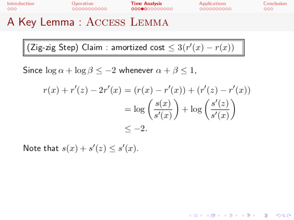
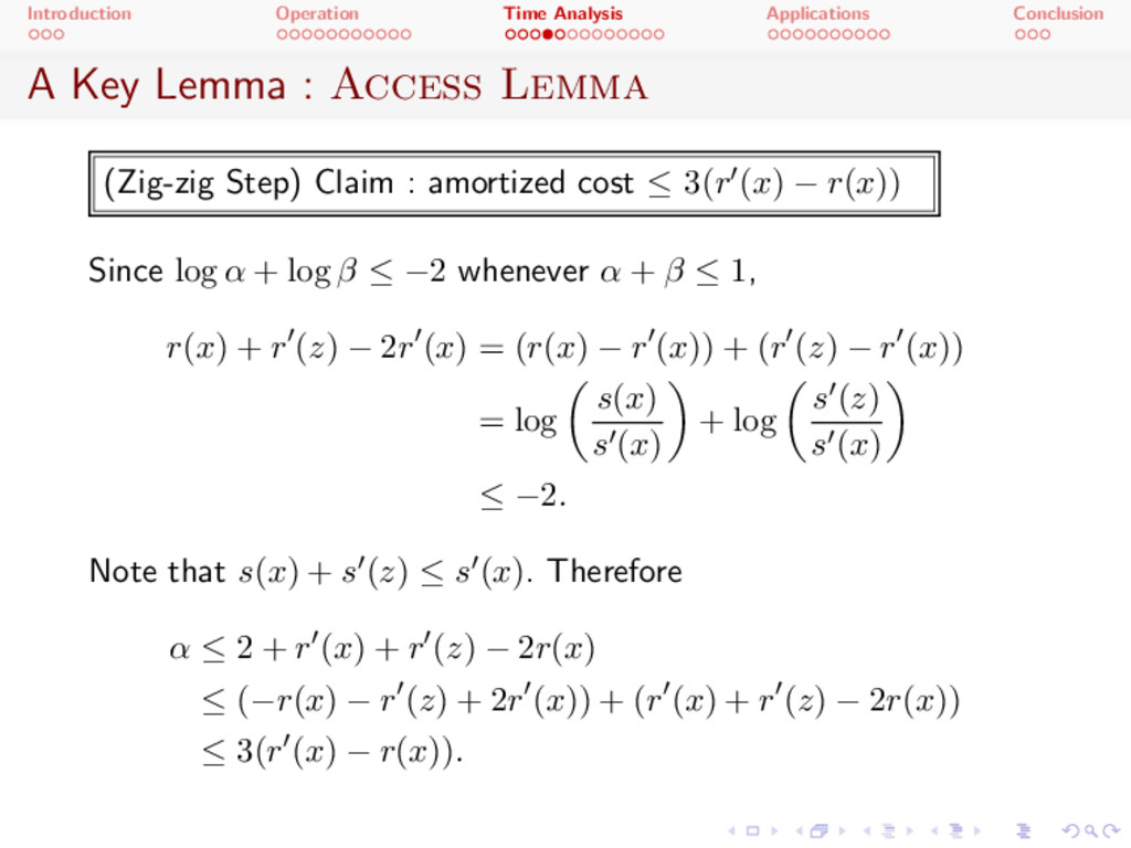
Access Lemma (Zig-zig Step) Claim : amortized cost 3( r0 ( x ) r ( x )) Since log ↵ + log 2 whenever ↵ + 1 , r ( x ) + r0 ( z ) 2 r0 ( x ) = ( r ( x ) r0 ( x )) + ( r0 ( z ) r0 ( x )) = log ✓ s ( x ) s0 ( x ) ◆ + log ✓ s0 ( z ) s0 ( x ) ◆ 2 . Note that s ( x ) + s0 ( z ) s0 ( x ) .
Access Lemma (Zig-zig Step) Claim : amortized cost 3( r0 ( x ) r ( x )) Since log ↵ + log 2 whenever ↵ + 1 , r ( x ) + r0 ( z ) 2 r0 ( x ) = ( r ( x ) r0 ( x )) + ( r0 ( z ) r0 ( x )) = log ✓ s ( x ) s0 ( x ) ◆ + log ✓ s0 ( z ) s0 ( x ) ◆ 2 . Note that s ( x ) + s0 ( z ) s0 ( x ) . Therefore ↵ 2 + r0 ( x ) + r0 ( z ) 2 r ( x ) ( r ( x ) r0 ( z ) + 2 r0 ( x )) + ( r0 ( x ) + r0 ( z ) 2 r ( x )) 3( r0 ( x ) r ( x )) .
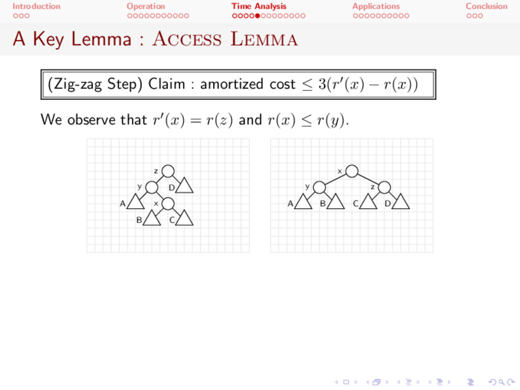
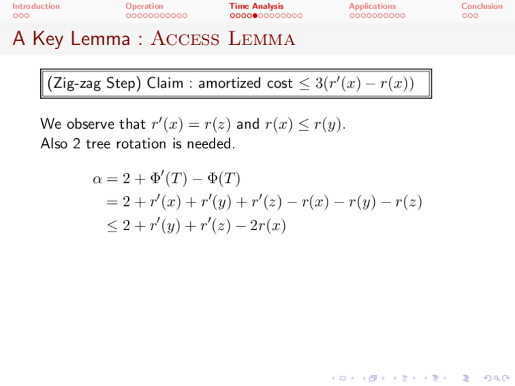
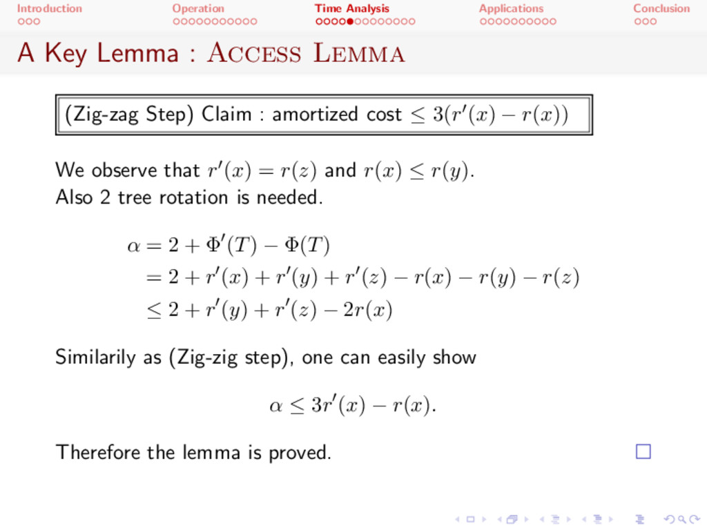
Access Lemma (Zig-zag Step) Claim : amortized cost 3( r0 ( x ) r ( x )) We observe that r0 ( x ) = r ( z ) and r ( x ) r ( y ) . x y z A B C D x y z A B C D
Access Lemma (Zig-zag Step) Claim : amortized cost 3( r0 ( x ) r ( x )) We observe that r0 ( x ) = r ( z ) and r ( x ) r ( y ) . Also 2 tree rotation is needed. ↵ = 2 + 0 ( T ) ( T ) = 2 + r0 ( x ) + r0 ( y ) + r0 ( z ) r ( x ) r ( y ) r ( z ) 2 + r0 ( y ) + r0 ( z ) 2 r ( x )
Access Lemma (Zig-zag Step) Claim : amortized cost 3( r0 ( x ) r ( x )) We observe that r0 ( x ) = r ( z ) and r ( x ) r ( y ) . Also 2 tree rotation is needed. ↵ = 2 + 0 ( T ) ( T ) = 2 + r0 ( x ) + r0 ( y ) + r0 ( z ) r ( x ) r ( y ) r ( z ) 2 + r0 ( y ) + r0 ( z ) 2 r ( x ) Similarily as (Zig-zig step), one can easily show ↵ 3 r0 ( x ) r ( x ) . Therefore the lemma is proved.
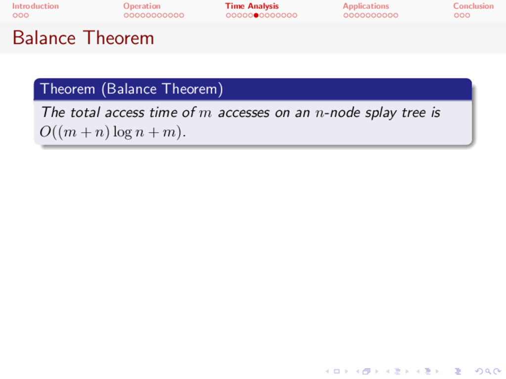
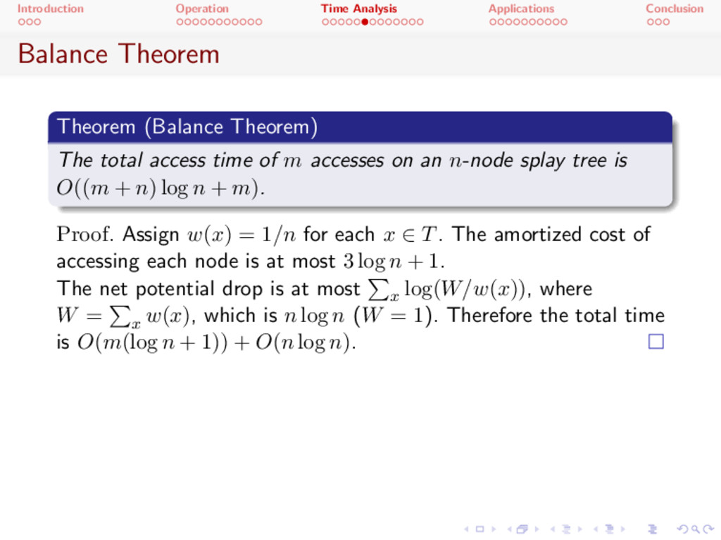
Theorem) The total access time of m accesses on an n-node splay tree is O (( m + n ) log n + m ) . Proof . Assign w ( x ) = 1 /n for each x 2 T. The amortized cost of accessing each node is at most 3 log n + 1 . The net potential drop is at most P x log( W/w ( x )) , where W = P x w ( x ) , which is n log n (W = 1 ). Therefore the total time is O ( m (log n + 1)) + O ( n log n ) .
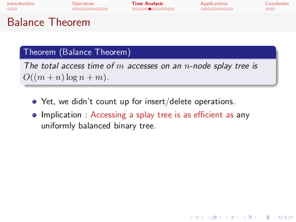
Theorem) The total access time of m accesses on an n-node splay tree is O (( m + n ) log n + m ) . Yet, we didn’t count up for insert/delete operations. Implication : Accessing a splay tree is as e cient as any uniformly balanced binary tree.
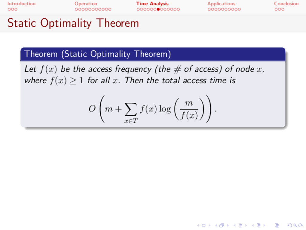
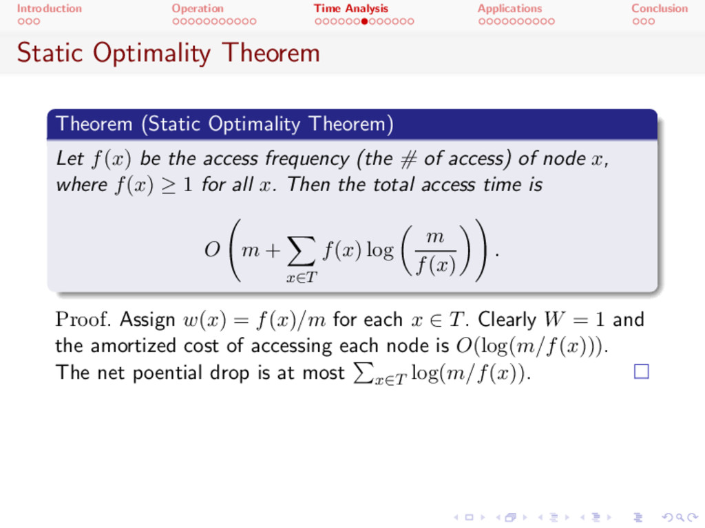
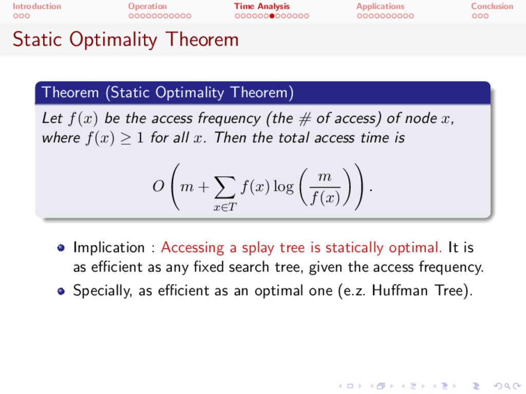
(Static Optimality Theorem) Let f ( x ) be the access frequency (the # of access) of node x, where f ( x ) 1 for all x. Then the total access time is O m + X x2T f ( x ) log ✓ m f ( x ) ◆! .
(Static Optimality Theorem) Let f ( x ) be the access frequency (the # of access) of node x, where f ( x ) 1 for all x. Then the total access time is O m + X x2T f ( x ) log ✓ m f ( x ) ◆! . Proof . Assign w ( x ) = f ( x ) /m for each x 2 T. Clearly W = 1 and the amortized cost of accessing each node is O (log( m/f ( x ))) . The net poential drop is at most P x2T log( m/f ( x )) .
(Static Optimality Theorem) Let f ( x ) be the access frequency (the # of access) of node x, where f ( x ) 1 for all x. Then the total access time is O m + X x2T f ( x ) log ✓ m f ( x ) ◆! . Implication : Accessing a splay tree is statically optimal. It is as e cient as any fixed search tree, given the access frequency. Specially, as e cient as an optimal one (e.z. Hu↵man Tree).
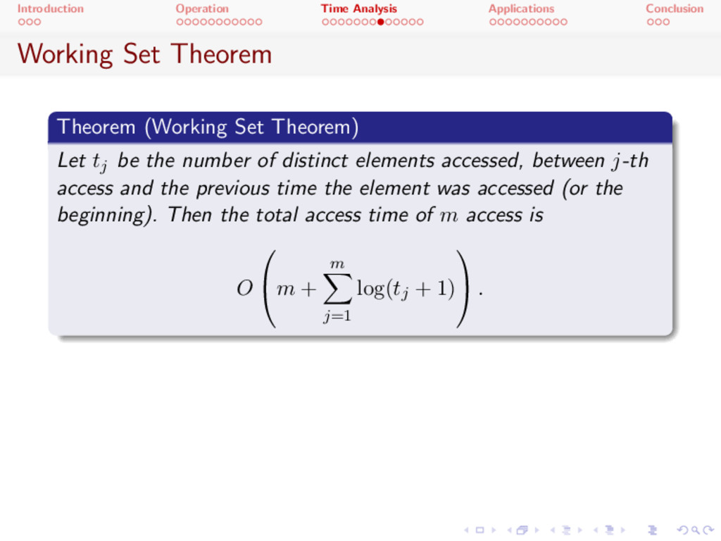
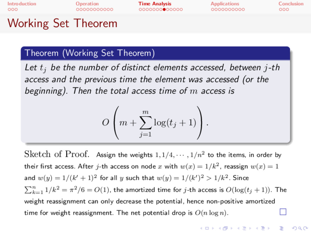
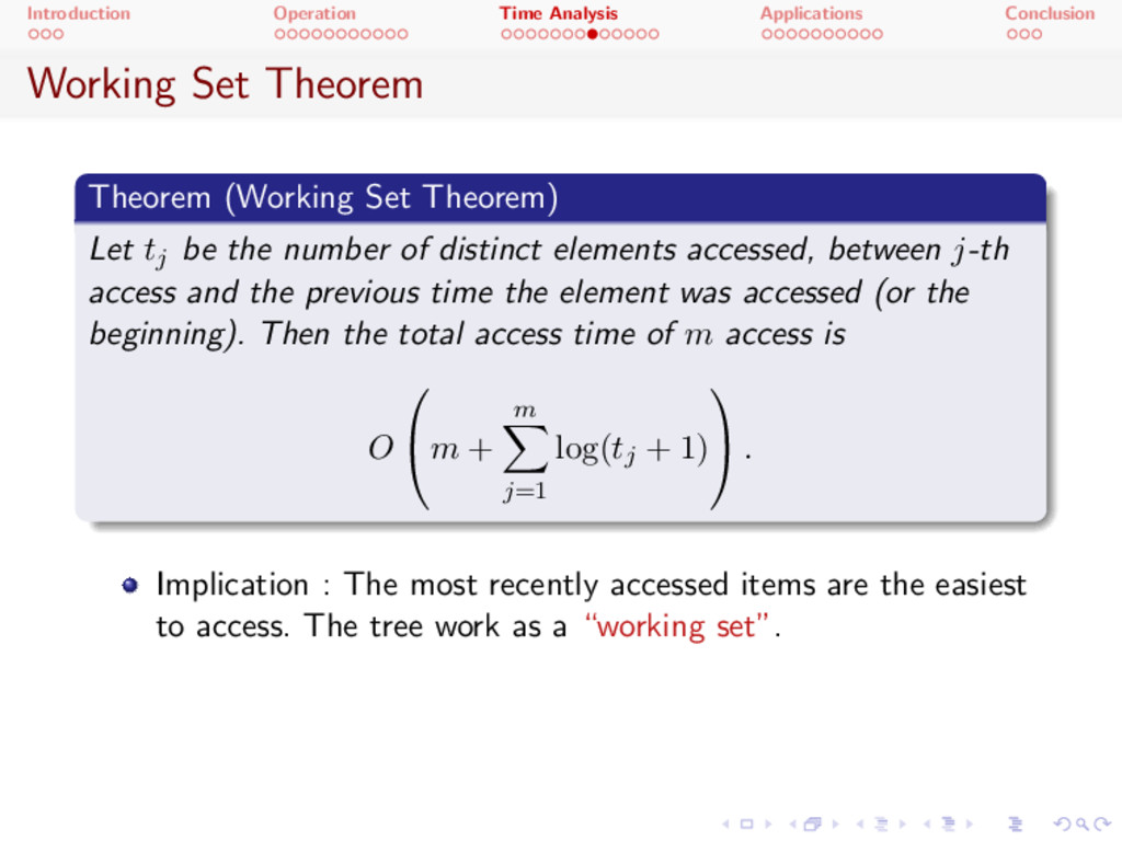
(Working Set Theorem) Let tj be the number of distinct elements accessed, between j-th access and the previous time the element was accessed (or the beginning). Then the total access time of m access is O 0 @m + m X j =1 log( tj + 1) 1 A .
(Working Set Theorem) Let tj be the number of distinct elements accessed, between j-th access and the previous time the element was accessed (or the beginning). Then the total access time of m access is O 0 @m + m X j =1 log( tj + 1) 1 A . Sketch of Proof . Assign the weights 1 , 1 / 4 , · · · , 1 /n2 to the items, in order by their first access. After j-th access on node x with w ( x ) = 1 /k2, reassign w ( x ) = 1 and w ( y ) = 1 / ( k0 + 1) 2 for all y such that w ( y ) = 1 / ( k0 ) 2 > 1 /k2. Since P n k =1 1 /k2 = ⇡2/ 6 = O (1) , the amortized time for j-th access is O (log( t j + 1)) . The weight reassignment can only decrease the potential, hence non-positive amortized time for weight reassignment. The net potential drop is O ( n log n ) .
(Working Set Theorem) Let tj be the number of distinct elements accessed, between j-th access and the previous time the element was accessed (or the beginning). Then the total access time of m access is O 0 @m + m X j =1 log( tj + 1) 1 A . Implication : The most recently accessed items are the easiest to access. The tree work as a “working set”.
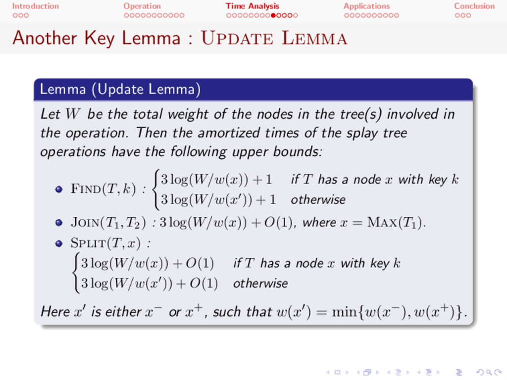
Update Lemma Lemma (Update Lemma) Let W be the total weight of the nodes in the tree(s) involved in the operation. Then the amortized times of the splay tree operations have the following upper bounds: Find( T, k ) : ( 3 log( W/w ( x )) + 1 if T has a node x with key k 3 log( W/w ( x0 )) + 1 otherwise Join( T1 , T2) : 3 log( W/w ( x )) + O (1) , where x = Max( T1) . Split( T, x ) : ( 3 log( W/w ( x )) + O (1) if T has a node x with key k 3 log( W/w ( x0 )) + O (1) otherwise Here x0 is either x or x+ , such that w ( x0 ) = min {w ( x ) , w ( x+) }.
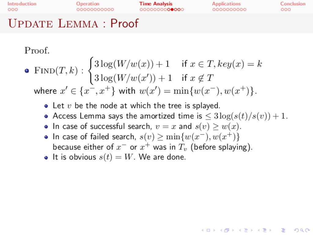
Proof. Find( T, k ) : ( 3 log( W/w ( x )) + 1 if x 2 T, key ( x ) = k 3 log( W/w ( x0 )) + 1 if x 62 T where x0 2 {x , x+} with w ( x0 ) = min {w ( x ) , w ( x+) }. Let v be the node at which the tree is splayed. Access Lemma says the amortized time is 3 log( s ( t ) /s ( v )) + 1 . In case of successful search, v = x and s ( v ) w ( x ) . In case of failed search, s ( v ) min {w ( x ) , w ( x+ ) } because either of x or x+ was in T v (before splaying). It is obvious s ( t ) = W. We are done.
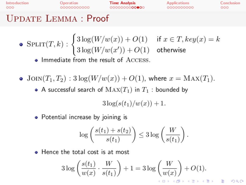
Split( T, k ) : ( 3 log( W/w ( x )) + O (1) if x 2 T, key ( x ) = k 3 log( W/w ( x0 )) + O (1) otherwise Immediate from the result of Access . Join( T 1 , T 2) : 3 log( W/w ( x )) + O (1) , where x = Max( T 1) . A successful search of Max( T1) in T1 : bounded by 3 log( s ( t1) /w ( x )) + 1 . Potential increase by joining is log ✓ s ( t1) + s ( t2) s ( t1) ◆ 3 log ✓ W s ( t1) ◆ . Hence the total cost is at most 3 log ✓ s ( t1) w ( x ) · W s ( t1) ◆ + 1 = 3 log ✓ W w ( x ) ◆ + O (1) .
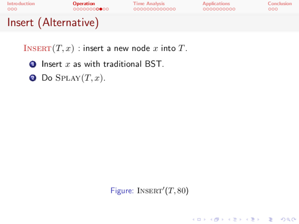
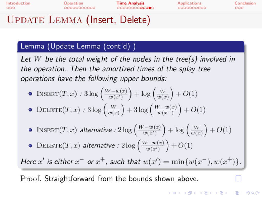
Lemma (Update Lemma (cont’d) ) Let W be the total weight of the nodes in the tree(s) involved in the operation. Then the amortized times of the splay tree operations have the following upper bounds: Insert( T, x ) : 3 log ⇣ W w ( x ) w ( x 0) ⌘ + log ⇣ W w ( x ) ⌘ + O (1) Delete( T, x ) : 3 log ⇣ W w ( x ) ⌘ + 3 log ⇣ W w ( x ) w ( x ) ⌘ + O (1) Insert( T, x ) alternative : 2 log ⇣ W w ( x ) w ( x 0) ⌘ + log ⇣ W w ( x ) ⌘ + O (1) Delete( T, x ) alternative : 2 log ⇣ W w ( x ) w ( x 0) ⌘ + O (1) Here x0 is either x or x+ , such that w ( x0 ) = min {w ( x ) , w ( x+) }. Proof . Straightforward from the bounds shown above.
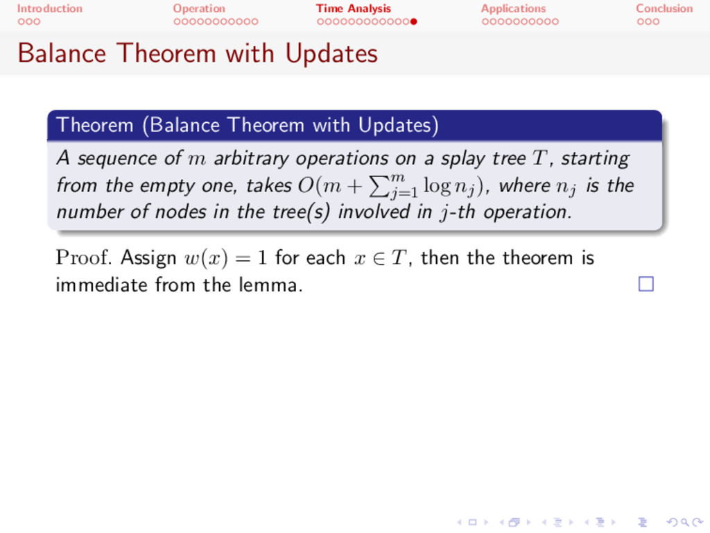
Theorem (Balance Theorem with Updates) A sequence of m arbitrary operations on a splay tree T, starting from the empty one, takes O ( m + Pm j =1 log nj ) , where nj is the number of nodes in the tree(s) involved in j-th operation. Proof . Assign w ( x ) = 1 for each x 2 T, then the theorem is immediate from the lemma.
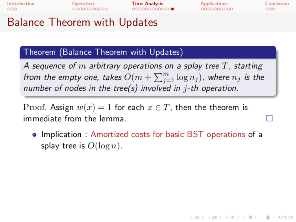
Theorem (Balance Theorem with Updates) A sequence of m arbitrary operations on a splay tree T, starting from the empty one, takes O ( m + Pm j =1 log nj ) , where nj is the number of nodes in the tree(s) involved in j-th operation. Proof . Assign w ( x ) = 1 for each x 2 T, then the theorem is immediate from the lemma. Implication : Amortized costs for basic BST operations of a splay tree is O (log n ) .
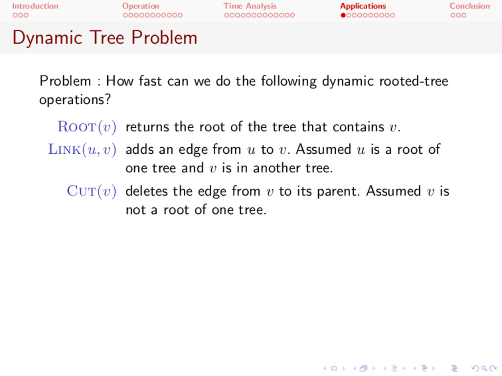
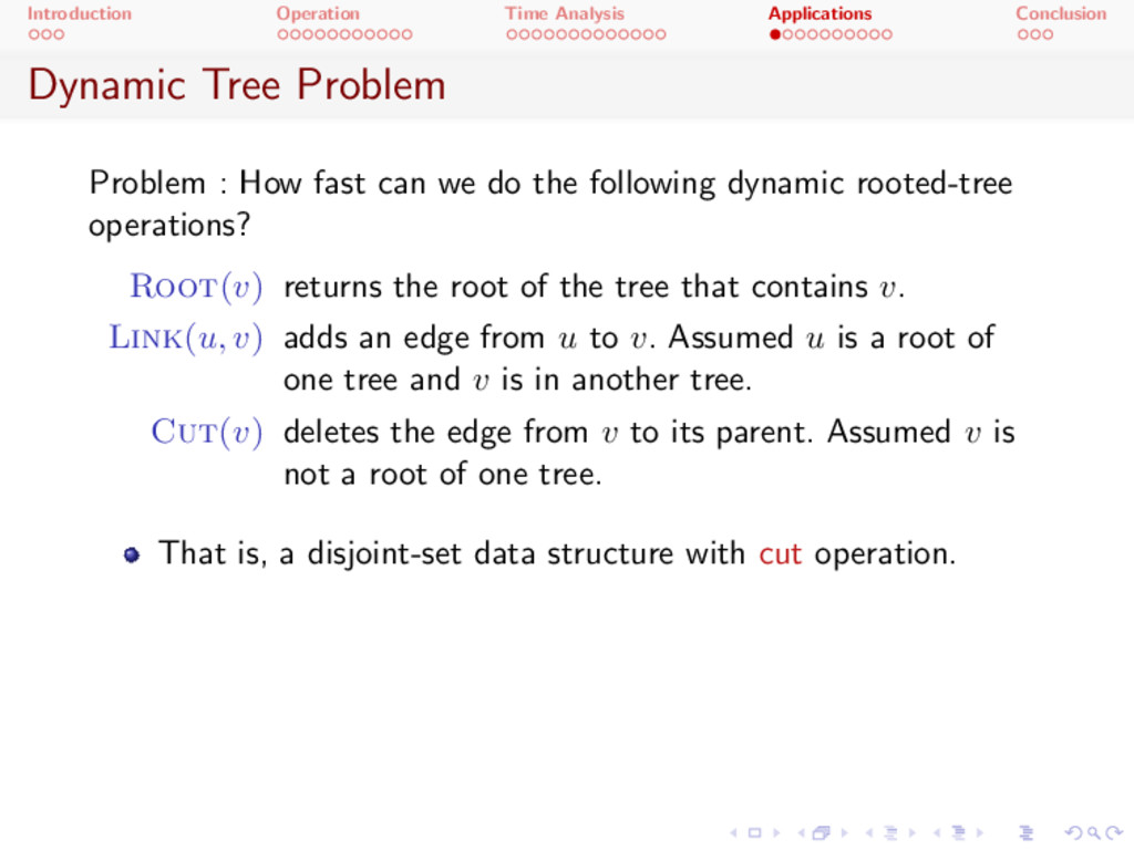
: How fast can we do the following dynamic rooted-tree operations? Root( v ) returns the root of the tree that contains v. Link( u, v ) adds an edge from u to v. Assumed u is a root of one tree and v is in another tree. Cut( v ) deletes the edge from v to its parent. Assumed v is not a root of one tree.
: How fast can we do the following dynamic rooted-tree operations? Root( v ) returns the root of the tree that contains v. Link( u, v ) adds an edge from u to v. Assumed u is a root of one tree and v is in another tree. Cut( v ) deletes the edge from v to its parent. Assumed v is not a root of one tree. That is, a disjoint-set data structure with cut operation.
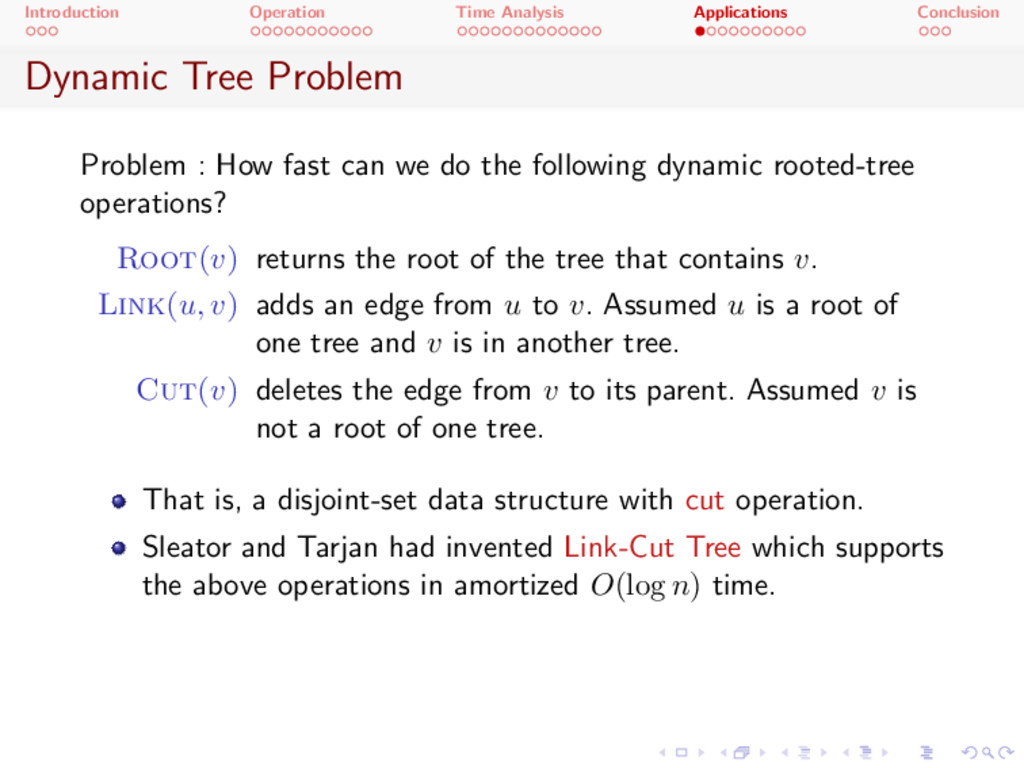
: How fast can we do the following dynamic rooted-tree operations? Root( v ) returns the root of the tree that contains v. Link( u, v ) adds an edge from u to v. Assumed u is a root of one tree and v is in another tree. Cut( v ) deletes the edge from v to its parent. Assumed v is not a root of one tree. That is, a disjoint-set data structure with cut operation. Sleator and Tarjan had invented Link-Cut Tree which supports the above operations in amortized O (log n ) time.
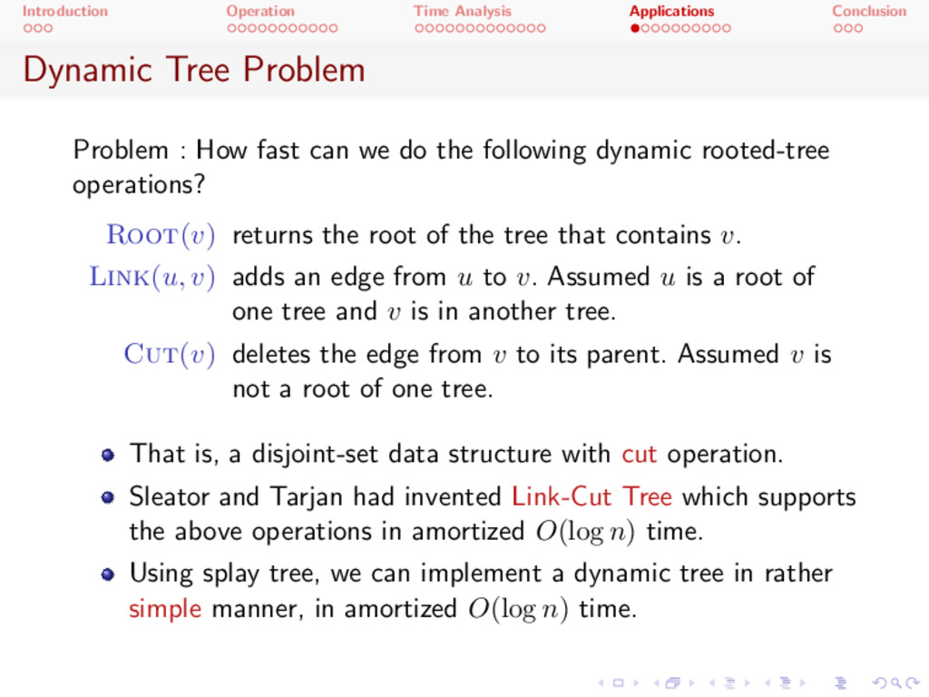
: How fast can we do the following dynamic rooted-tree operations? Root( v ) returns the root of the tree that contains v. Link( u, v ) adds an edge from u to v. Assumed u is a root of one tree and v is in another tree. Cut( v ) deletes the edge from v to its parent. Assumed v is not a root of one tree. That is, a disjoint-set data structure with cut operation. Sleator and Tarjan had invented Link-Cut Tree which supports the above operations in amortized O (log n ) time. Using splay tree, we can implement a dynamic tree in rather simple manner, in amortized O (log n ) time.
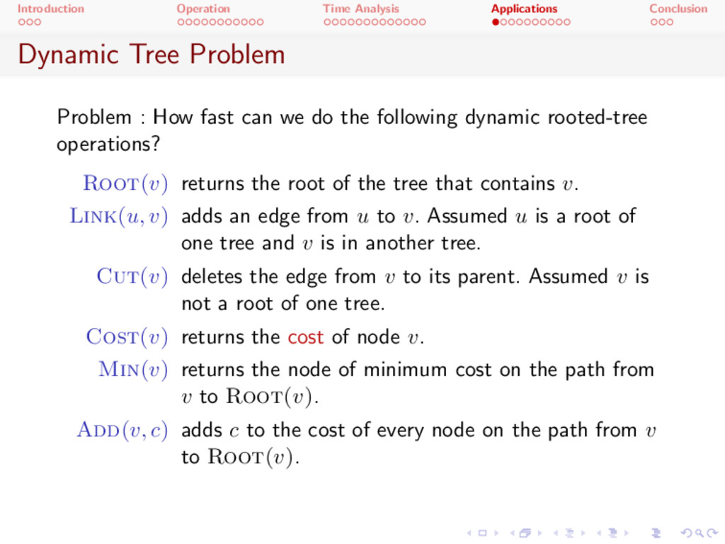
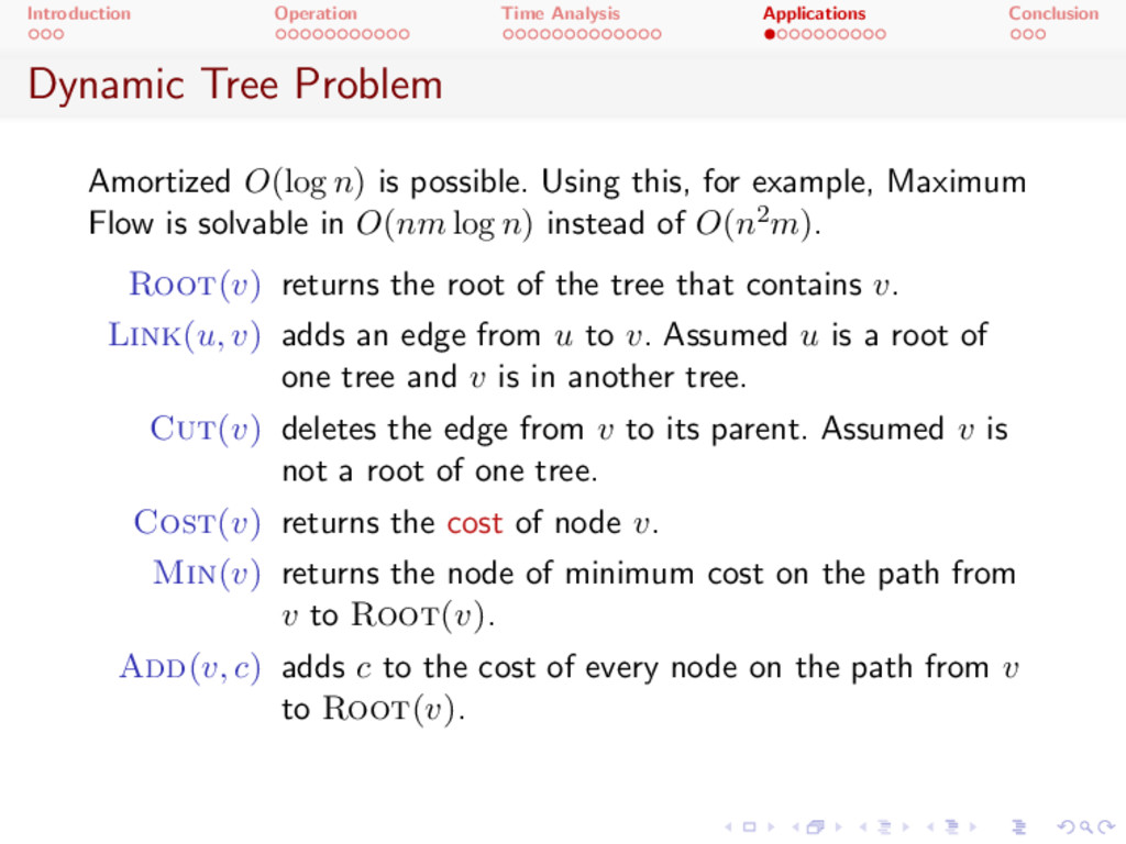
: How fast can we do the following dynamic rooted-tree operations? Root( v ) returns the root of the tree that contains v. Link( u, v ) adds an edge from u to v. Assumed u is a root of one tree and v is in another tree. Cut( v ) deletes the edge from v to its parent. Assumed v is not a root of one tree. Cost( v ) returns the cost of node v. Min( v ) returns the node of minimum cost on the path from v to Root( v ) . Add( v, c ) adds c to the cost of every node on the path from v to Root( v ) .
O (log n ) is possible. Using this, for example, Maximum Flow is solvable in O ( nm log n ) instead of O ( n2 m ) . Root( v ) returns the root of the tree that contains v. Link( u, v ) adds an edge from u to v. Assumed u is a root of one tree and v is in another tree. Cut( v ) deletes the edge from v to its parent. Assumed v is not a root of one tree. Cost( v ) returns the cost of node v. Min( v ) returns the node of minimum cost on the path from v to Root( v ) . Add( v, c ) adds c to the cost of every node on the path from v to Root( v ) .
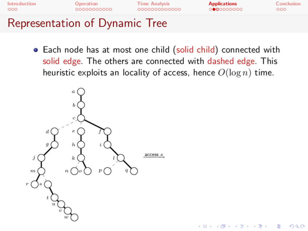
Each node has at most one child (solid child) connected with solid edge. The others are connected with dashed edge. This heuristic exploits an locality of access, hence O (log n ) time. a b c d e f g h i j k l m n o p q r s t u v w access s !
Each node has at most one child (solid child) connected with solid edge. The others are connected with dashed edge. This heuristic exploits an locality of access, hence O (log n ) time. a b c d e f g h i j k l m n o p q r s t u v w access s ! a b c d e f g h i j k l m n o p q r s t u v w
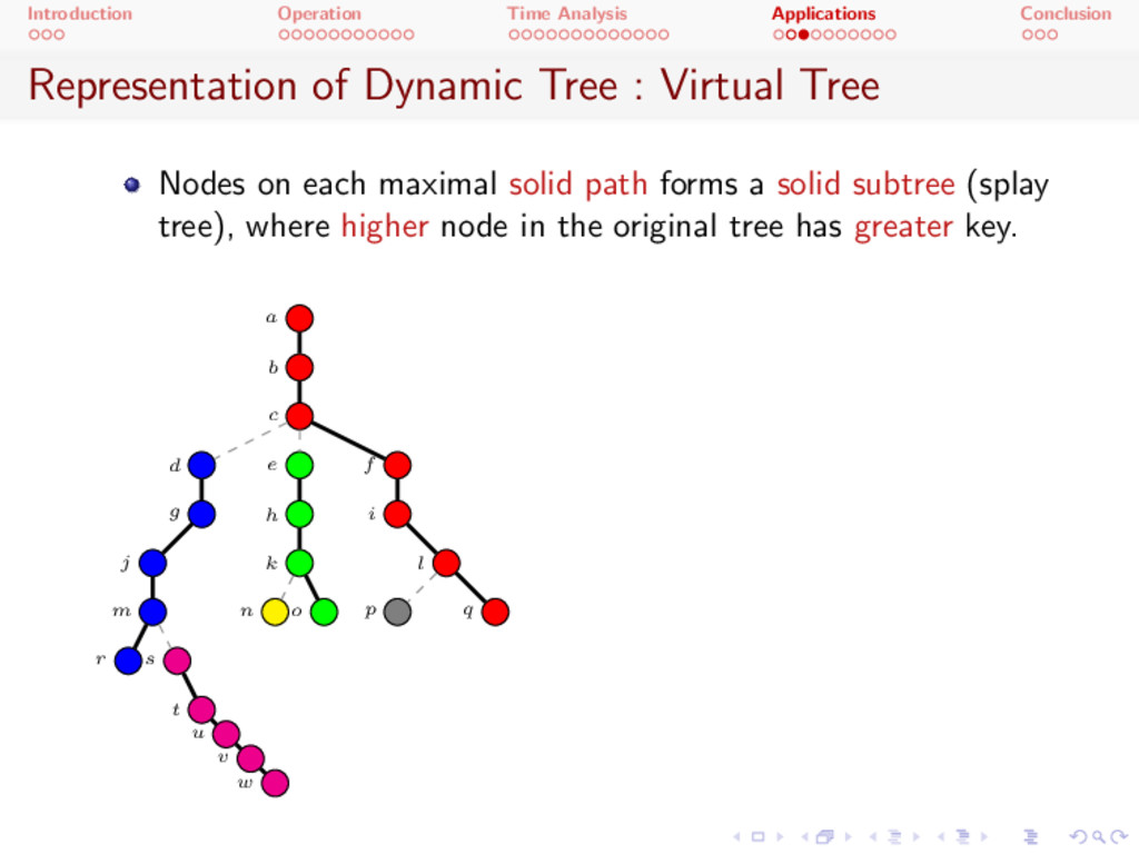
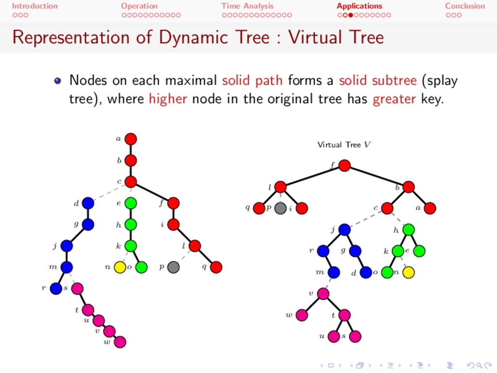
: Virtual Tree Nodes on each maximal solid path forms a solid subtree (splay tree), where higher node in the original tree has greater key. a b c d e f g h i j k l m n o p q r s t u v w
: Virtual Tree Nodes on each maximal solid path forms a solid subtree (splay tree), where higher node in the original tree has greater key. a b c d e f g h i j k l m n o p q r s t u v w Virtual Tree V f l b q p i c a j r g d m v w t u s h k e o n
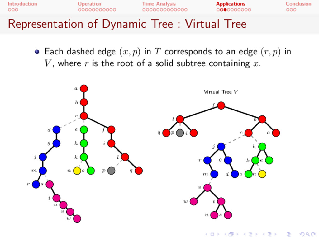
: Virtual Tree Each dashed edge ( x, p ) in T corresponds to an edge ( r, p ) in V , where r is the root of a solid subtree containing x. a b c d e f g h i j k l m n o p q r s t u v w Virtual Tree V f l b q p i c a j r g d m v w t u s h k e o n
) We have to restruct the virtual tree V , as if v was accessed in the original tree T. Note that solid paths and solid subtrees change. Access operation in Dynamic Tree, which encapsulates Splay operation in (a subtree of) Virtual tree
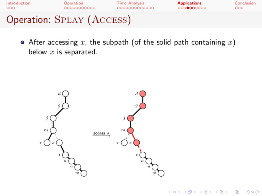
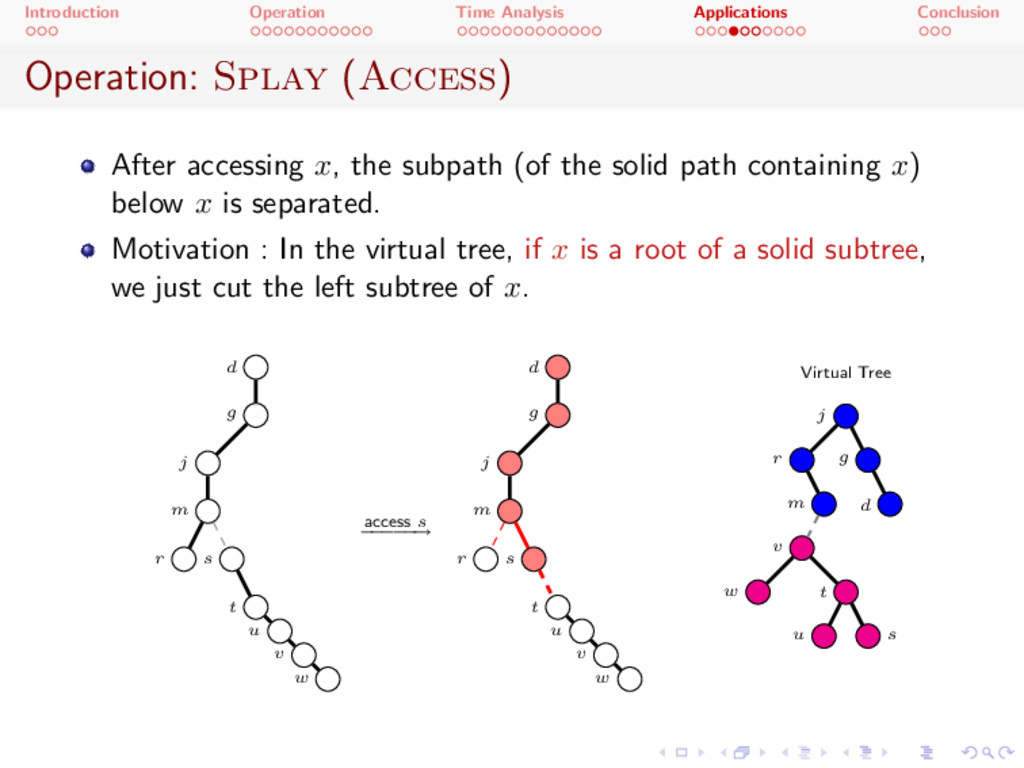
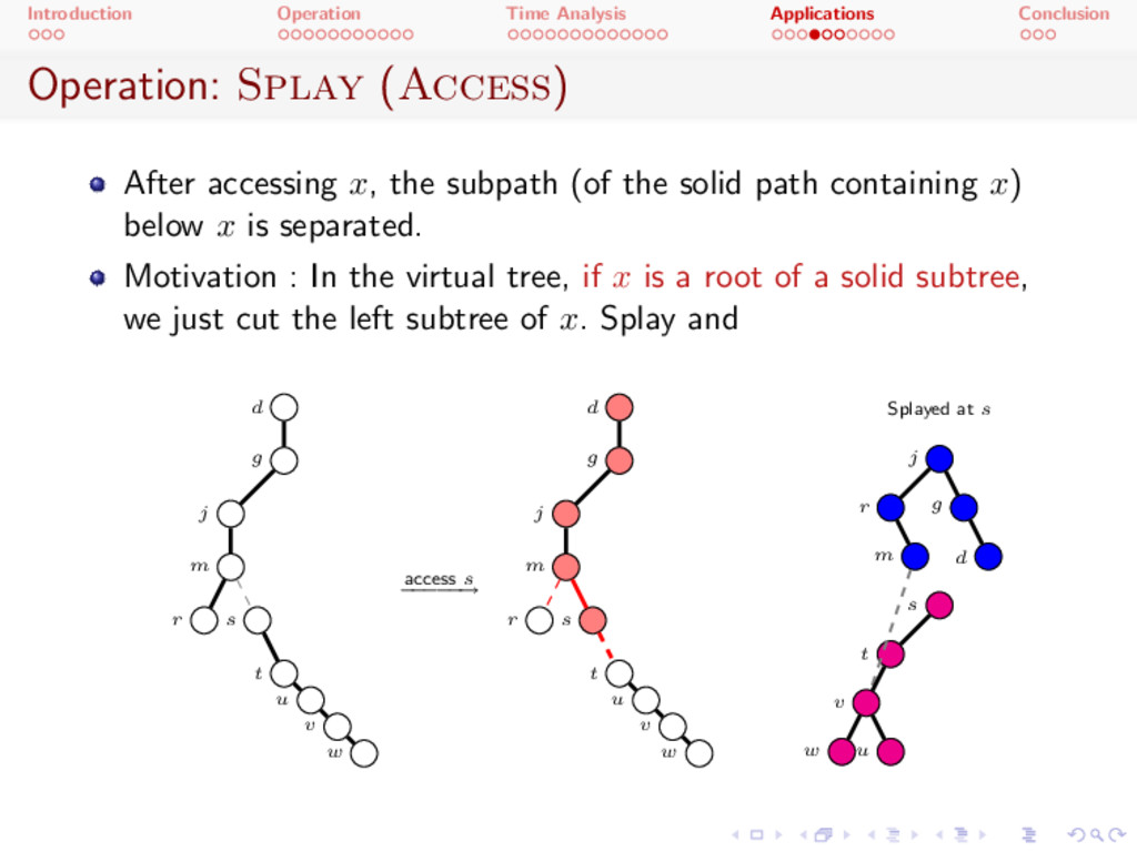
) After accessing x, the subpath (of the solid path containing x) below x is separated. Motivation : In the virtual tree, if x is a root of a solid subtree, we just cut the left subtree of x. d g j m r s t u v w access s ! d g j m r s t u v w Virtual Tree j r g d m v w t u s
) After accessing x, the subpath (of the solid path containing x) below x is separated. Motivation : In the virtual tree, if x is a root of a solid subtree, we just cut the left subtree of x. Splay and d g j m r s t u v w access s ! d g j m r s t u v w Splayed at s j r g d m s t v w u
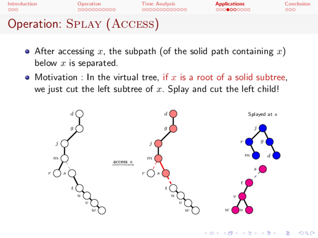
) After accessing x, the subpath (of the solid path containing x) below x is separated. Motivation : In the virtual tree, if x is a root of a solid subtree, we just cut the left subtree of x. Splay and cut the left child! d g j m r s t u v w access s ! d g j m r s t u v w Splayed at s j r g d m s t v w u
Access in dynamic tree is just doing Splay within the entire virtual tree. Please do not confuse ‘splaying’ in a virtual tree with ‘splaying’ in a solid subtree, which is just a subroutine.
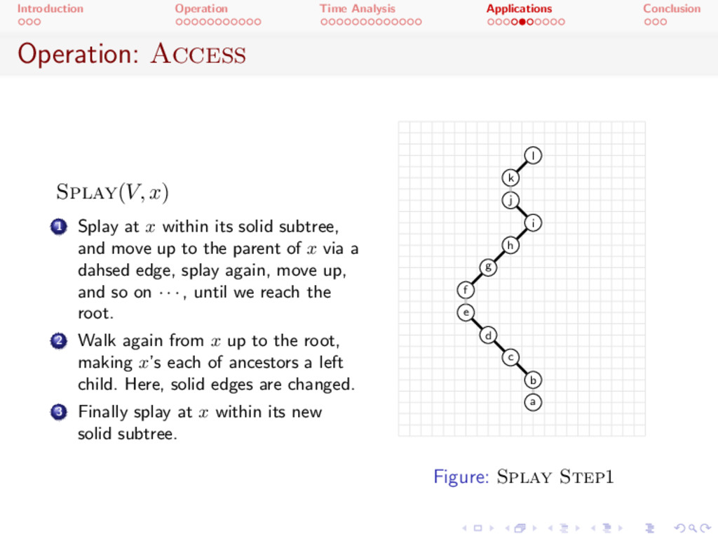
x ) 1 Splay at x within its solid subtree, and move up to the parent of x via a dahsed edge, splay again, move up, and so on · · · , until we reach the root. 2 Walk again from x up to the root, making x ’s each of ancestors a left child. Here, solid edges are changed. 3 Finally splay at x within its new solid subtree. Figure: Splay Step1
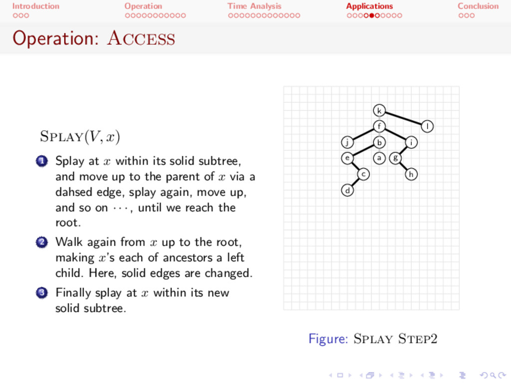
x ) 1 Splay at x within its solid subtree, and move up to the parent of x via a dahsed edge, splay again, move up, and so on · · · , until we reach the root. 2 Walk again from x up to the root, making x ’s each of ancestors a left child. Here, solid edges are changed. 3 Finally splay at x within its new solid subtree. Figure: Splay Step2
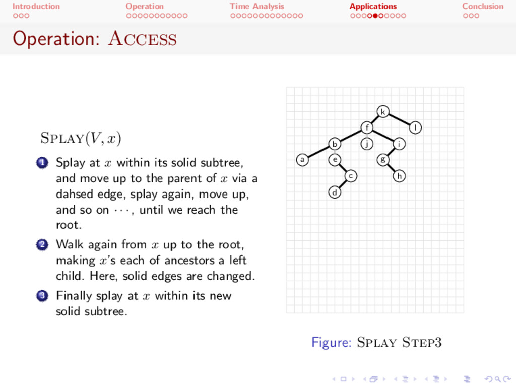
x ) 1 Splay at x within its solid subtree, and move up to the parent of x via a dahsed edge, splay again, move up, and so on · · · , until we reach the root. 2 Walk again from x up to the root, making x ’s each of ancestors a left child. Here, solid edges are changed. 3 Finally splay at x within its new solid subtree. Figure: Splay Step3
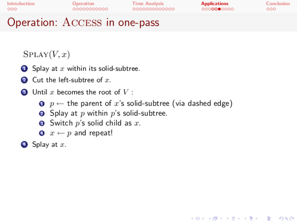
Splay( V, x ) 1 Splay at x within its solid-subtree. 2 Cut the left-subtree of x . 3 Until x becomes the root of V : 1 p the parent of x’s solid-subtree (via dashed edge) 2 Splay at p within p’s solid-subtree. 3 Switch p’s solid child as x. 4 x p and repeat! 4 Splay at x .
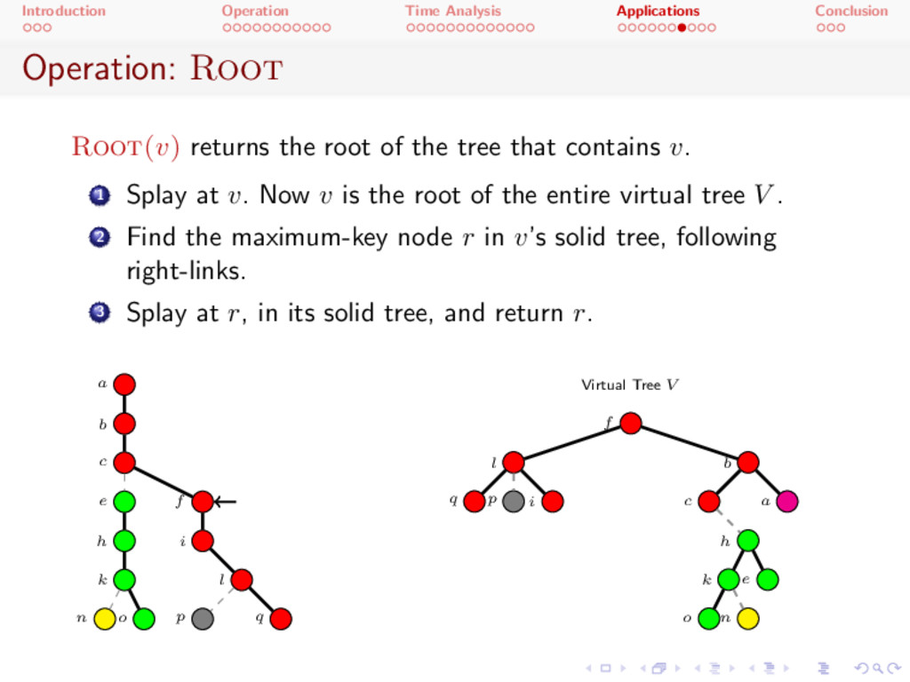
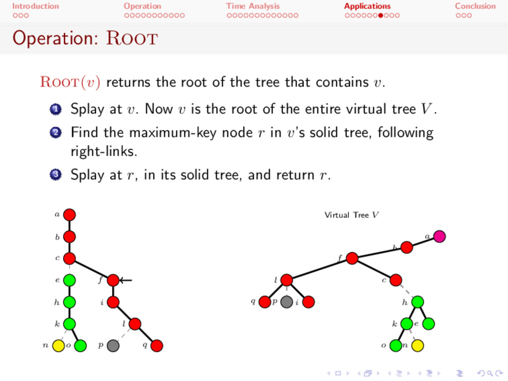
) returns the root of the tree that contains v. 1 Splay at v. Now v is the root of the entire virtual tree V . 2 Find the maximum-key node r in v’s solid tree, following right-links. 3 Splay at r, in its solid tree, and return r. a b c e f h i k l n o p q Virtual Tree V f l b q p i c a h k e o n
) returns the root of the tree that contains v. 1 Splay at v. Now v is the root of the entire virtual tree V . 2 Find the maximum-key node r in v’s solid tree, following right-links. 3 Splay at r, in its solid tree, and return r. a b c e f h i k l n o p q Virtual Tree V f l b q p i c a h k e o n
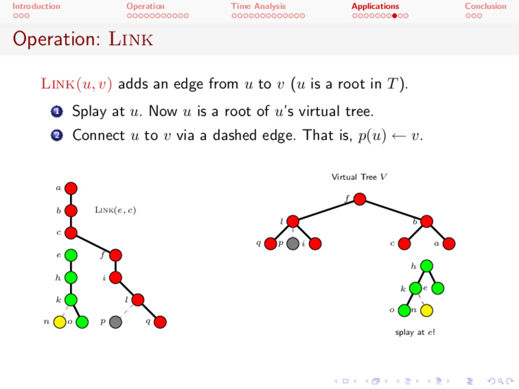
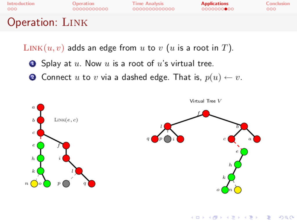
v ) adds an edge from u to v (u is a root in T). 1 Splay at u. Now u is a root of u’s virtual tree. 2 Connect u to v via a dashed edge. That is, p ( u ) v. a b c e f h i k l n o p q Link ( e, c ) Virtual Tree V f l b q p i c a h k e o n splay at e !
v ) adds an edge from u to v (u is a root in T). 1 Splay at u. Now u is a root of u’s virtual tree. 2 Connect u to v via a dashed edge. That is, p ( u ) v. a b c e f h i k l n o p q Link ( e, c ) Virtual Tree V f l b q p i c a e h k o n
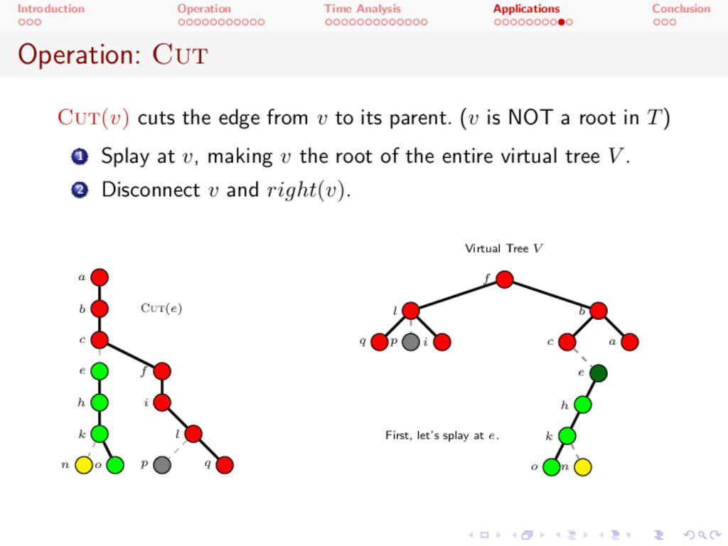
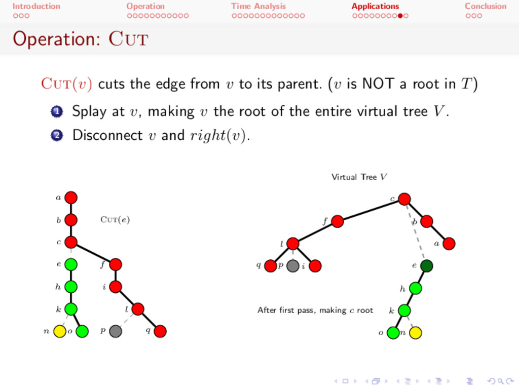
) cuts the edge from v to its parent. (v is NOT a root in T) 1 Splay at v, making v the root of the entire virtual tree V . 2 Disconnect v and right ( v ) . a b c e f h i k l n o p q Cut ( e ) Virtual Tree V First, let’s splay at e . f l q p i c a b e h k o n
) cuts the edge from v to its parent. (v is NOT a root in T) 1 Splay at v, making v the root of the entire virtual tree V . 2 Disconnect v and right ( v ) . a b c e f h i k l n o p q Cut ( e ) Virtual Tree V After first pass, making c root f l q p i c a b e h k o n
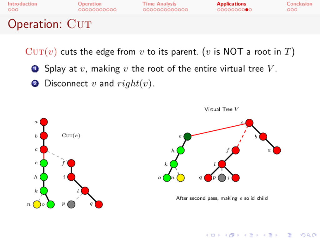
) cuts the edge from v to its parent. (v is NOT a root in T) 1 Splay at v, making v the root of the entire virtual tree V . 2 Disconnect v and right ( v ) . a b c e f h i k l n o p q Cut ( e ) Virtual Tree V After second pass, making e solid child f l q p i c a b e h k o n
) cuts the edge from v to its parent. (v is NOT a root in T) 1 Splay at v, making v the root of the entire virtual tree V . 2 Disconnect v and right ( v ) . a b c e f h i k l n o p q Cut ( e ) Virtual Tree V After third pass, making e root f l q p i c b a e h k o n
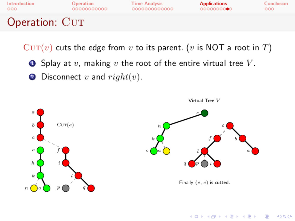
) cuts the edge from v to its parent. (v is NOT a root in T) 1 Splay at v, making v the root of the entire virtual tree V . 2 Disconnect v and right ( v ) . a b c e f h i k l n o p q Cut ( e ) Virtual Tree V Finally ( e, c ) is cutted. f l q p i c b a e h k o n
operations are done in amortized O (log n ) time. Another potential analysis : in the virtual tree V , weight w ( x ) = 1 for each node x 2 V size s ( x ) := the number of its descendants (the sum of weight), including subtrees connected via dashed edges. rank r ( x ) := log s ( x ) (binary logarithm) potential ( V ) := 2 P x in V r ( x ) A single splay operation costs amortized O (log n ) . The first pass costs 6 log n + k, where k is the depth of x after the first pass (the number of zig cases). The second pass costs zero since there is no rotations. For the third pass, each of the k rotations is charged two to take account for k rotations in the first pass, hence 6 log n + 2 . Now the total amortized time is O (log n ) .
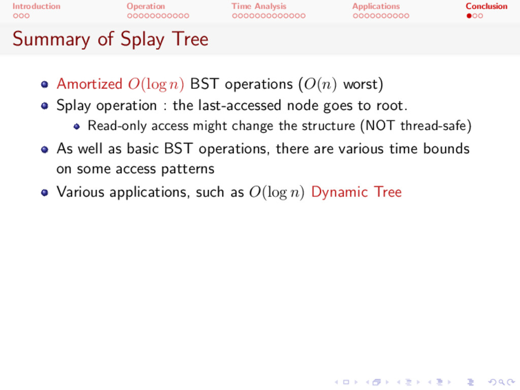
Amortized O (log n ) BST operations (O ( n ) worst) Splay operation : the last-accessed node goes to root. Read-only access might change the structure (NOT thread-safe) As well as basic BST operations, there are various time bounds on some access patterns Various applications, such as O (log n ) Dynamic Tree
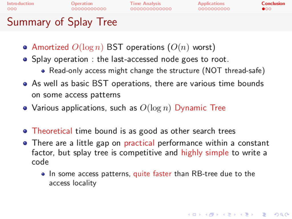
Amortized O (log n ) BST operations (O ( n ) worst) Splay operation : the last-accessed node goes to root. Read-only access might change the structure (NOT thread-safe) As well as basic BST operations, there are various time bounds on some access patterns Various applications, such as O (log n ) Dynamic Tree Theoretical time bound is as good as other search trees There are a little gap on practical performance within a constant factor, but splay tree is competitive and highly simple to write a code In some access patterns, quite faster than RB-tree due to the access locality
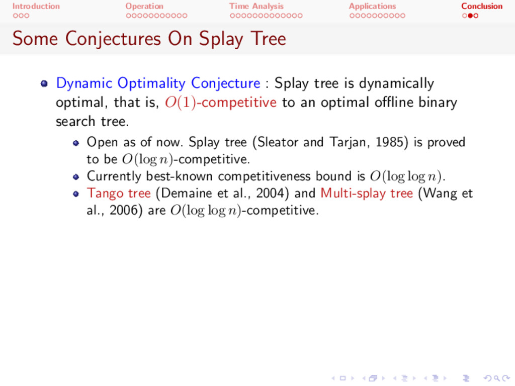
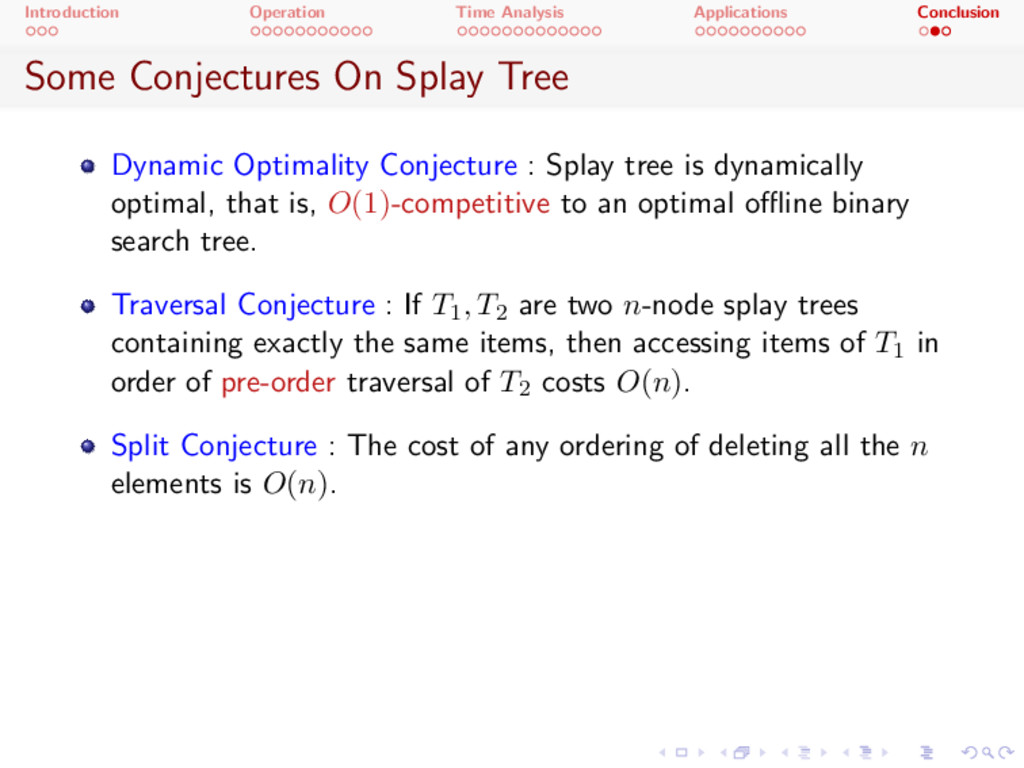
Tree Dynamic Optimality Conjecture : Splay tree is dynamically optimal, that is, O (1) -competitive to an optimal o✏ine binary search tree. Open as of now. Splay tree (Sleator and Tarjan, 1985) is proved to be O (log n ) -competitive. Currently best-known competitiveness bound is O (log log n ) . Tango tree (Demaine et al., 2004) and Multi-splay tree (Wang et al., 2006) are O (log log n ) -competitive.
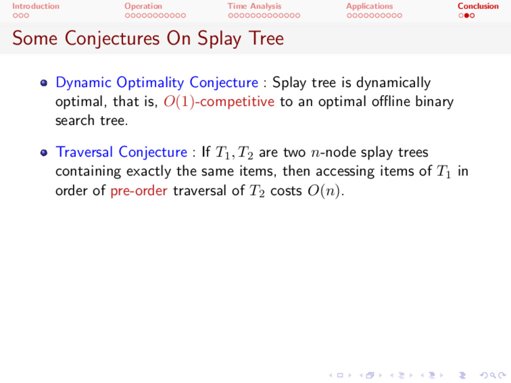
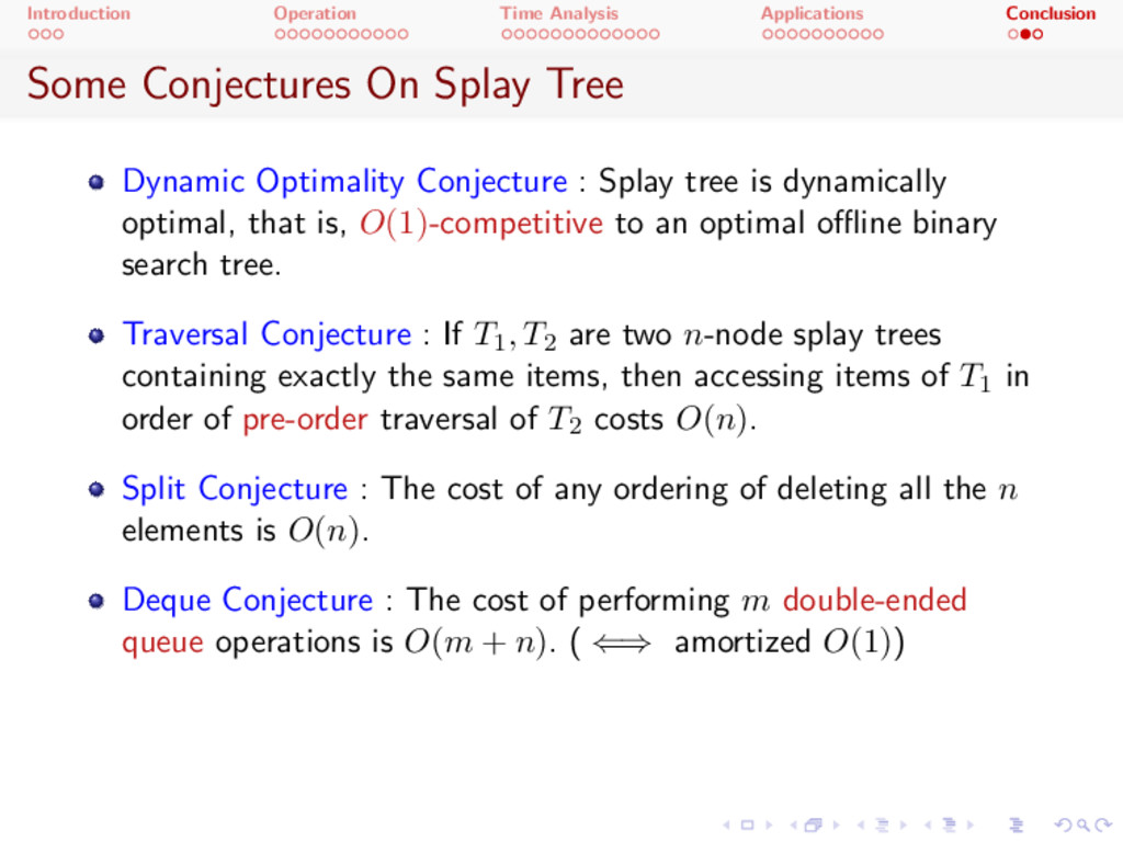
Tree Dynamic Optimality Conjecture : Splay tree is dynamically optimal, that is, O (1) -competitive to an optimal o✏ine binary search tree. Traversal Conjecture : If T 1 , T 2 are two n-node splay trees containing exactly the same items, then accessing items of T 1 in order of pre-order traversal of T 2 costs O ( n ) .
Tree Dynamic Optimality Conjecture : Splay tree is dynamically optimal, that is, O (1) -competitive to an optimal o✏ine binary search tree. Traversal Conjecture : If T 1 , T 2 are two n-node splay trees containing exactly the same items, then accessing items of T 1 in order of pre-order traversal of T 2 costs O ( n ) . Split Conjecture : The cost of any ordering of deleting all the n elements is O ( n ) .
Tree Dynamic Optimality Conjecture : Splay tree is dynamically optimal, that is, O (1) -competitive to an optimal o✏ine binary search tree. Traversal Conjecture : If T 1 , T 2 are two n-node splay trees containing exactly the same items, then accessing items of T 1 in order of pre-order traversal of T 2 costs O ( n ) . Split Conjecture : The cost of any ordering of deleting all the n elements is O ( n ) . Deque Conjecture : The cost of performing m double-ended queue operations is O ( m + n ) . ( () amortized O (1) )