[CS Foundation] AIML - 5 - Deep Learning

Transcript

1. Deep Learning Foundations Jie-Han Chen 2018/08/16 @ National Cheng Kung University and X-Village, Taiwan
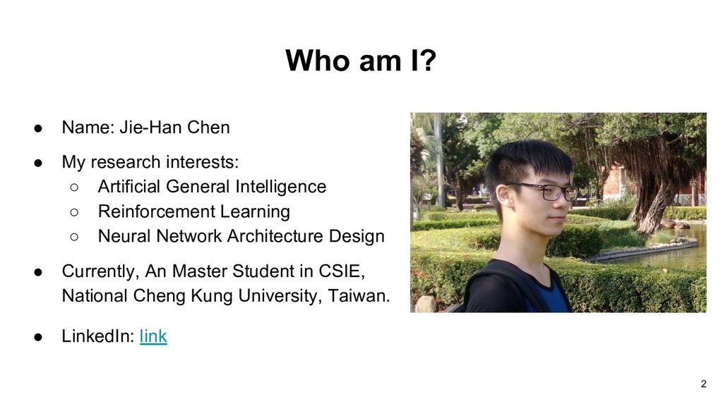
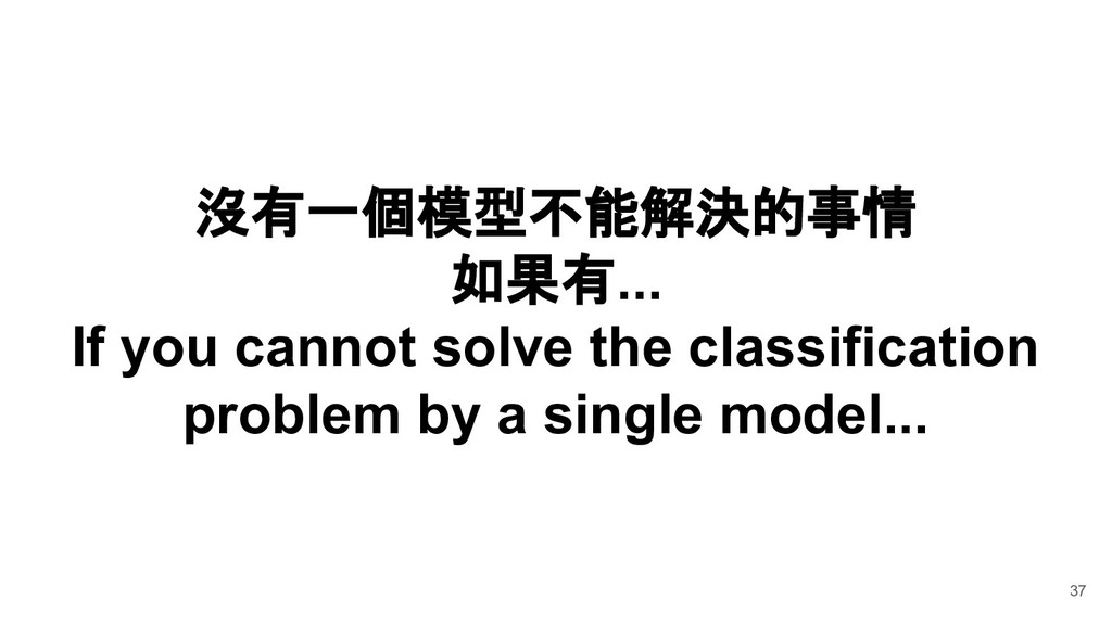
2. Who am I? • Name: Jie-Han Chen • My research interests: ◦ Artificial General Intelligence ◦ Reinforcement Learning ◦ Neural Network Architecture Design • Currently, An Master Student in CSIE, National Cheng Kung University, Taiwan. • LinkedIn: link 2
3. The revolution Recent years, deep learning has provided impressing results in many domains: • Computer Vision • Speech and Text Recognition • Decision making policy and Control • Modification and Generation 3
4. Computer Vision Object detection Redmon et al., YOLO(2016) Semantic Segmentation Long et al., FCN(2015) 4
5. Speech and Text Recognition Language Translation Speech Recognition and Chatbot 5
6. Decision Making Policy and Control Gaming (AI development) Robotics 6
7. Modification and Generation 7 click!
8. Interesting application 8 Quickdraw: https://quickdraw.withgoogle.com/ AutoDraw: https://www.autodraw.com/
9. They were all built by the Magic 9
11. Let’s unveil the mysteries of Deep Learning 11
12. You don’t need to pick up all contents in this lecture. Just keep something in mind, when training neural network. 12
13. Outline • The inspiration of artificial neural network • Perceptron & multi-layer perceptrons • Neural network • Optimization and learning algorithm • Tips for training neural network • Reference • Resources 13
14. “At least two ingredients are necessary for the advancement of a technology: • Concept • Implementation” -- (quoted from Neural Network Design) 14
15. quoted from Neural Network Design, 2nd edition. 由神經科學(neuroscience)得 知神經元包含以下元素: • 神經細胞本體 Cell Body • 樹突 Dendrites • 軸突 Axon • 突觸 Synapse The inspiration of Artificial Neural Network Biological Neurons 15
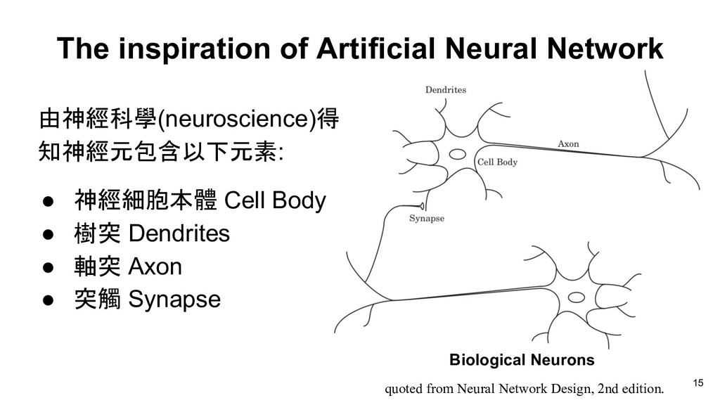
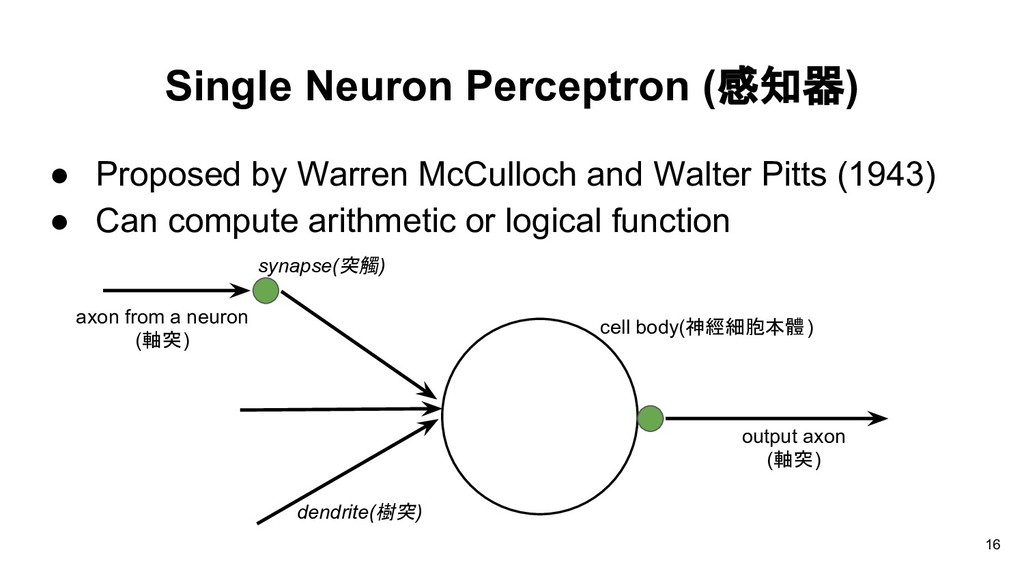
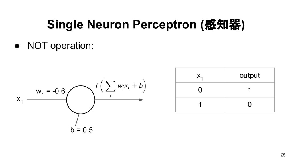
16. Single Neuron Perceptron (感知器) • Proposed by Warren McCulloch and Walter Pitts (1943) • Can compute arithmetic or logical function axon from a neuron (軸突) synapse(突觸) dendrite(樹突) output axon (軸突) cell body(神經細胞本體) 16
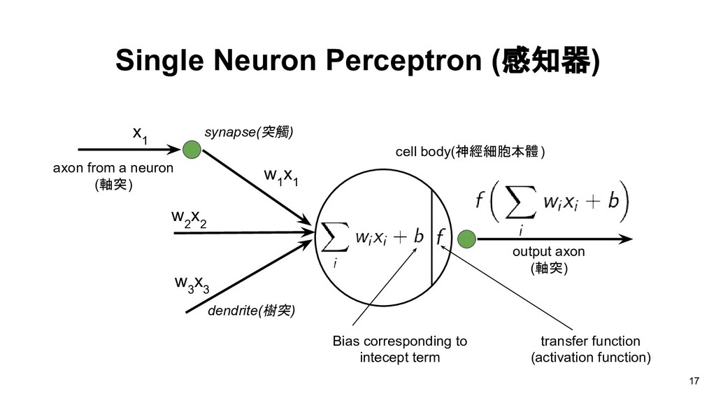
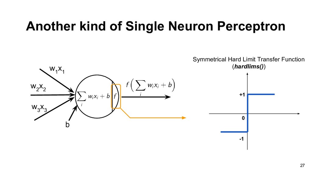
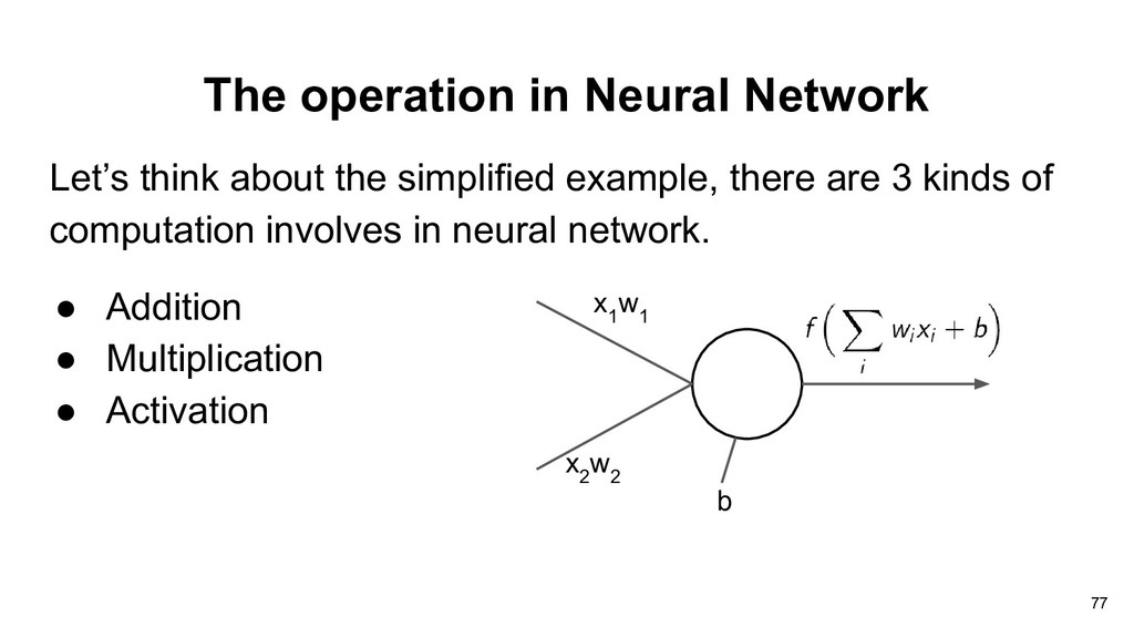
17. Single Neuron Perceptron (感知器) w 2 x 2 w 3 x 3 x 1 axon from a neuron (軸突) synapse(突觸) w 1 x 1 dendrite(樹突) cell body(神經細胞本體) output axon (軸突) Bias corresponding to intecept term transfer function (activation function) 17
18. Single Neuron Perceptron (感知器) +1 0 Hard Limit Transfer Function (hardlim() or sgn()) w 1 x 1 b w 2 x 2 w 3 x 3 18
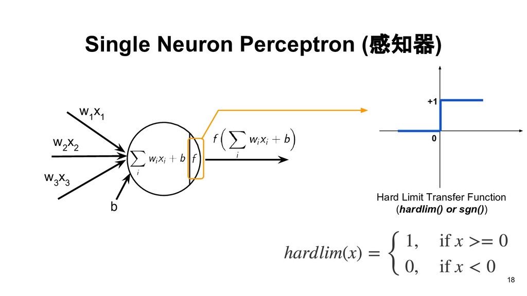
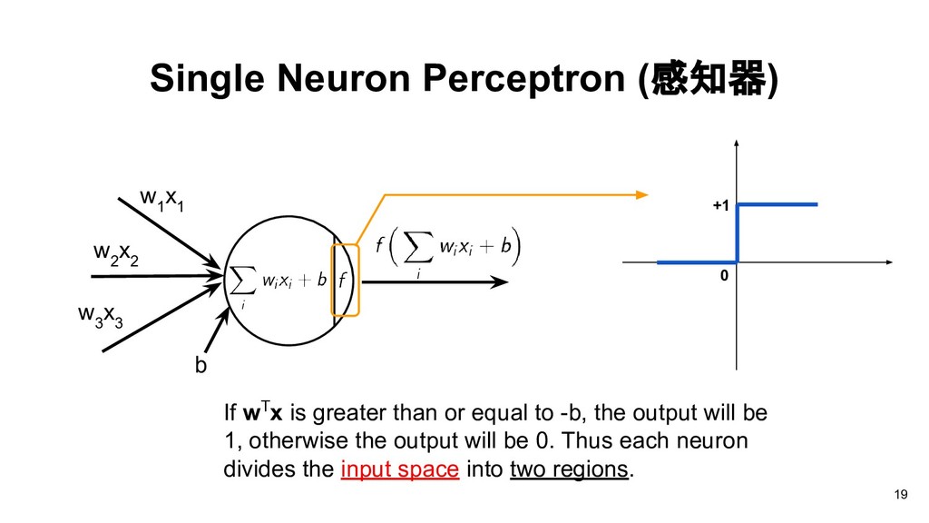
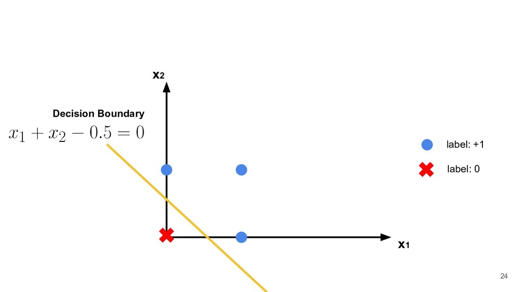
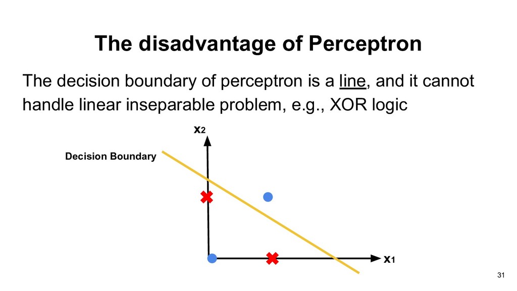
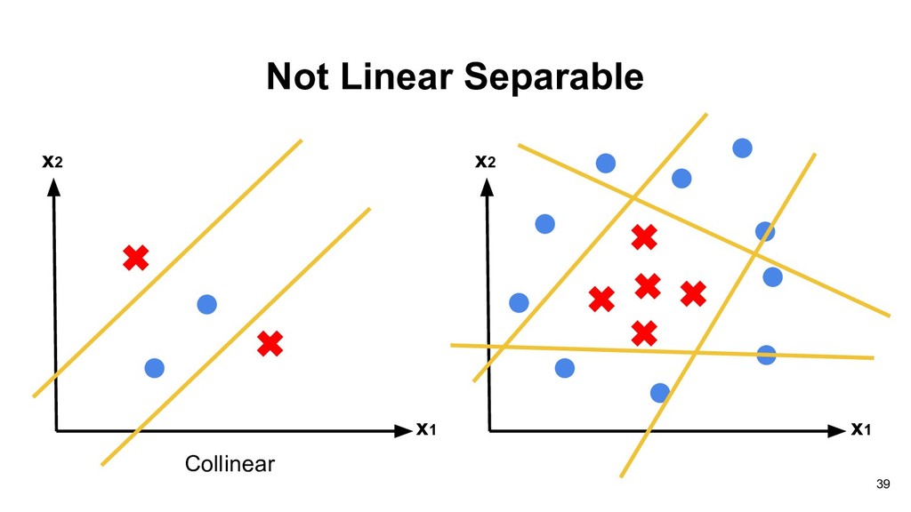
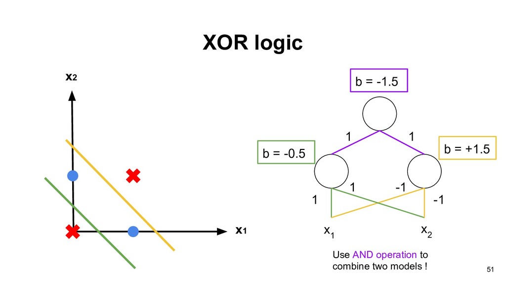
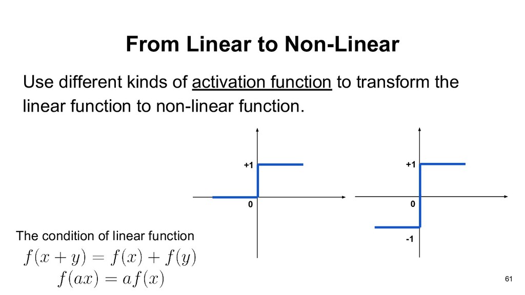
19. Single Neuron Perceptron (感知器) +1 0 If wTx is greater than or equal to -b, the output will be 1, otherwise the output will be 0. Thus each neuron divides the input space into two regions. w 1 x 1 w 2 x 2 w 3 x 3 b 19
20. Single Neuron Perceptron (感知器) x2 x1 label: +1 label: 0 Decision Boundary 20 weight vector (point to positive side)
21. • AND operation: Single Neuron Perceptron (感知器) x 1 x 2 output 0 0 0 0 1 0 1 0 0 1 1 1 x 1 x 2 w 1 = 1 w 2 = 1 b = -1.5 21
22. x2 Decision Boundary x1 label: +1 label: 0 22
23. • OR operation: Single Neuron Perceptron (感知器) x 1 x 2 output 0 0 0 0 1 1 1 0 1 1 1 1 x 1 x 2 w 1 = 1 w 2 = 1 b = -0.5 23
24. x2 Decision Boundary x1 label: +1 label: 0 24
25. • NOT operation: Single Neuron Perceptron (感知器) x 1 w 1 = -0.6 b = 0.5 x 1 output 0 1 1 0 25
26. We can change transfer function to build different models. 26
27. Another kind of Single Neuron Perceptron w 2 x 2 w 3 x 3 w 1 x 1 +1 0 -1 Symmetrical Hard Limit Transfer Function (hardlims()) b 27
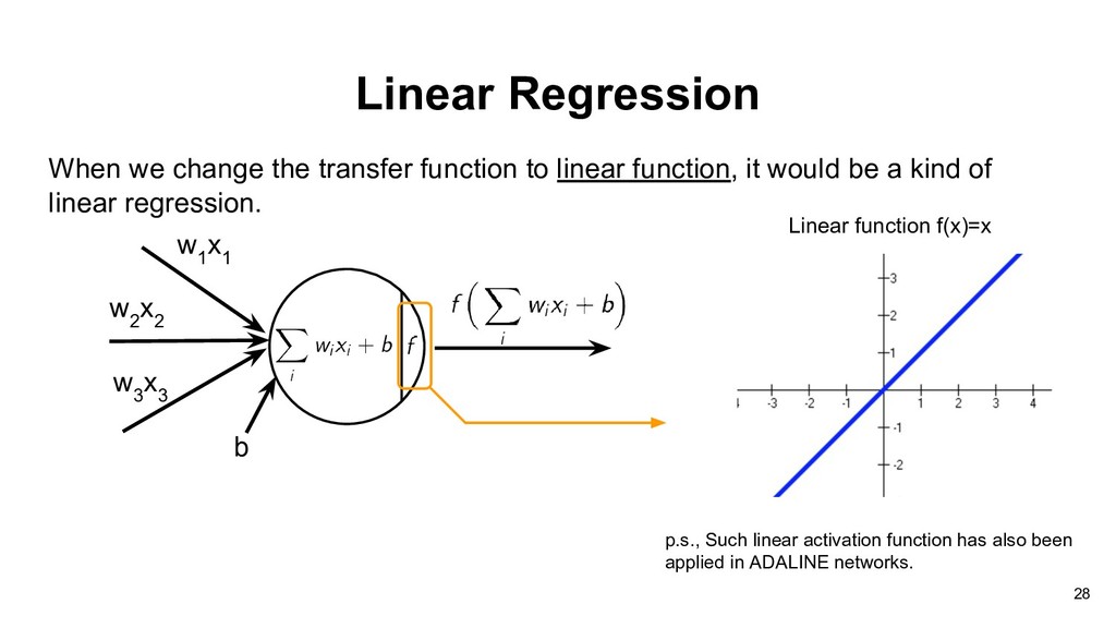
28. When we change the transfer function to linear function, it would be a kind of linear regression. Linear Regression Linear function f(x)=x p.s., Such linear activation function has also been applied in ADALINE networks. w 2 x 2 w 3 x 3 w 1 x 1 b 28
29. Logistic Regression Logistic function w 2 x 2 w 3 x 3 w 1 x 1 b 29
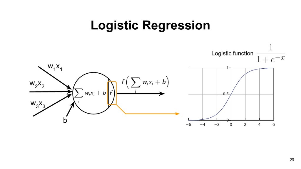
30. Learning algorithm of Perceptron We won’t cover the Perceptron Learning Algorithm(PLA) here. if you have strong interest about the learning algorithm, just notice that the learning algorithm would be different with different transfer functions, hardlim and hardlims. • hardlim: see the details in “Neural network design” in Chapter4 (formula 4.34, 4.35) • hardlims: see the details in “Learning from data” in Chapter1 (formula 1.3) • You also can write down the loss function and use derivative to derive the learning algorithm. 30
31. The disadvantage of Perceptron The decision boundary of perceptron is a line, and it cannot handle linear inseparable problem, e.g., XOR logic x1 x2 Decision Boundary 31
32. Questions? 32
33. Linear Separable V.S. Not Linear Separable 我們可以將 資料 分成兩個類型: Linear Separable, Not Linear Separable。 • Linear Separable: 資料本身可以由直線分割。 • Not Linear Separable: 資料本身不可由直線分割。 33
34. Linear Separable x2 x2 x1 x1 34
35. Linear Separable g(x) g(x) x1 x1 x2 x2 35
36. Not Linear Separable x1 x2 x1 x2 Collinear 共線 36
37. 沒有一個模型不能解決的事情 如果有... If you cannot solve the classification problem by a single model... 37
38. 就結合更多模型 Just give it more models! 38
39. Not Linear Separable x1 x2 x1 x2 Collinear 39
40. Let’s introduce the notation before giving you the concept of neural network 40
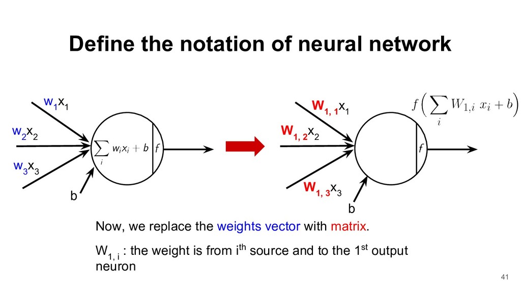
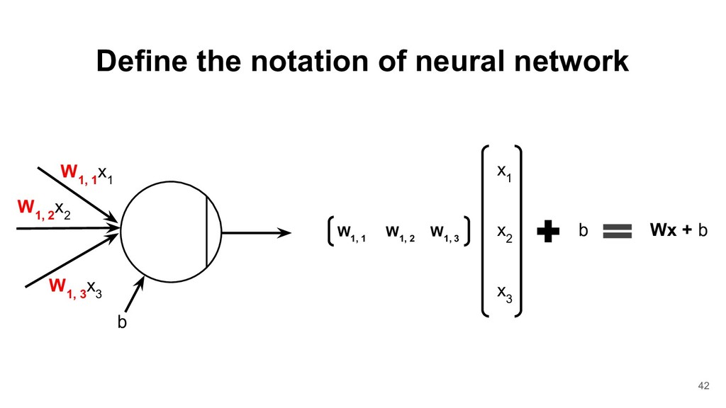
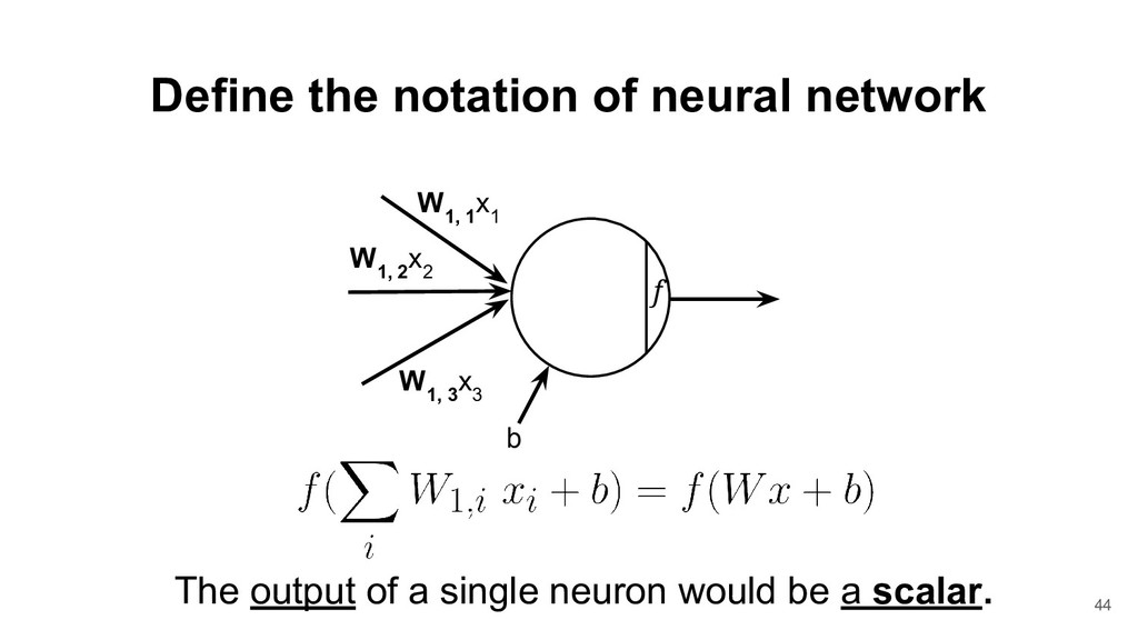
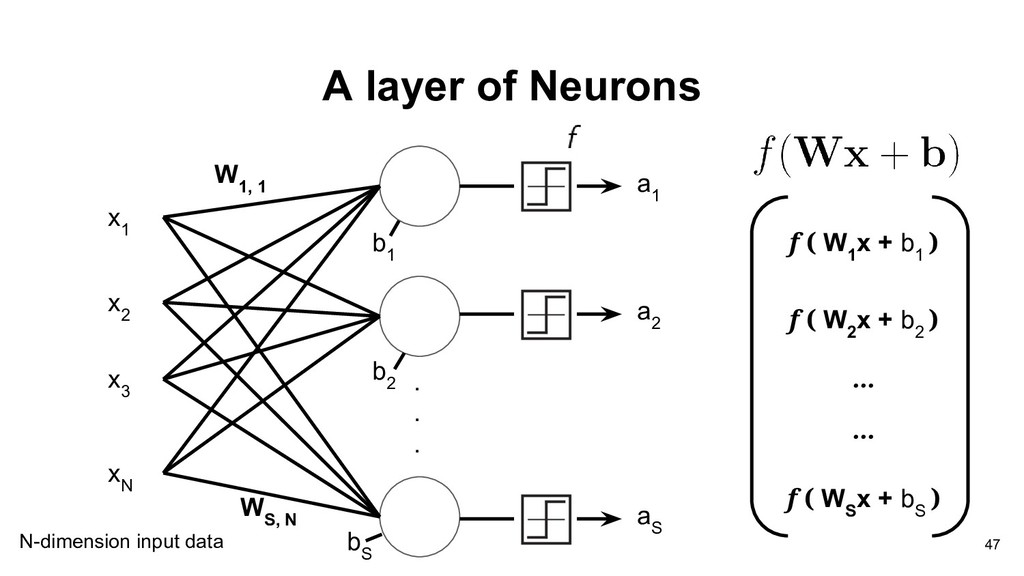
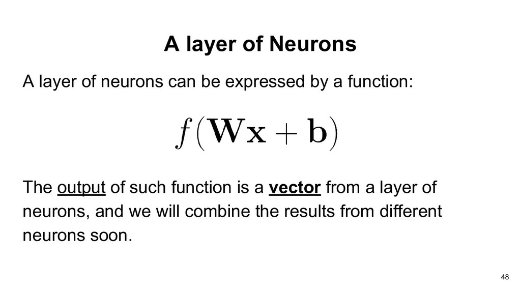
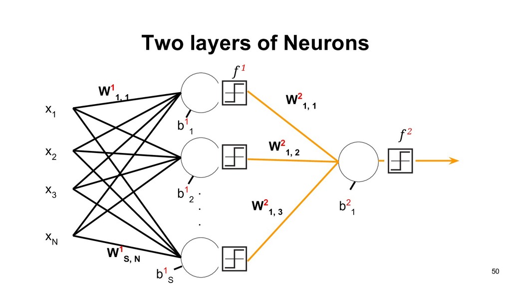
41. Define the notation of neural network W 1, 2 x 2 W 1, 3 x 3 W 1, 1 x 1 Now, we replace the weights vector with matrix. W 1, i : the weight is from ith source and to the 1st output neuron b w 2 x 2 w 3 x 3 w 1 x 1 b 41
42. Define the notation of neural network W 1, 2 x 2 W 1, 3 x 3 W 1, 1 x 1 b W 1, 1 W 1, 2 W 1, 3 x 1 x 2 x 3 b Wx + b 42
43. Define the notation of neural network W 1, 2 x 2 W 1, 3 x 3 W 1, 1 x 1 b W 1, 1 W 1, 2 W 1, 3 x 1 x 2 x 3 b f( Wx + b ) f f 43
44. Define the notation of neural network W 1, 2 x 2 W 1, 3 x 3 W 1, 1 x 1 b f The output of a single neuron would be a scalar. 44
45. A layer of Neurons - Single Neuron Perceptron each output denotes a single model(decision boundary) . . . x 1 x 2 x 3 x N N-dimension input data a 1 a 2 a S W 1, 1 W 1, 2 W 1, 3 W 1, N 1 W 1, 0 = b 1 45
46. A layer of Neurons - Single Neuron Perceptron . . . x 1 x 2 x 3 x N N-dimension input data a 1 a 2 a S W 1, 1 W 1, 2 W 1, 3 W 1, N 1 W 1, 0 = b 1 Notice: we add the input of bias here! 46
47. A layer of Neurons . . . x 1 x 2 x 3 x N N-dimension input data a 1 a 2 a S W 1, 1 W S, N b 1 b 2 b S f ( W 1 x + b 1 ) f ( W 2 x + b 2 ) f ( W S x + b S ) ... ... 47
48. A layer of neurons can be expressed by a function: The output of such function is a vector from a layer of neurons, and we will combine the results from different neurons soon. A layer of Neurons 48
49. Two layers of Neurons . . . x 1 x 2 x 3 x N W 1, 1 W S, N b 1 b 2 b S We can combine different models into a more powerful single model by adding another layer of neurons. f 49
50. Two layers of Neurons . . . x 1 x 2 x 3 x N W1 1, 1 W1 S, N b1 1 b1 2 b1 S W2 1, 1 W2 1, 2 W2 1, 3 b2 1 f 1 f 2 50
51. XOR logic x2 51 x1 x 1 x 2 1 1 -1 -1 b = -0.5 b = +1.5 1 1 b = -1.5 Use AND operation to combine two models !
52. Multi-Layer Perceptron (MLP) Input layer hidden layer output layer 52
53. Multi-Layer Perceptron (MLP) We also can add more hidden layers in MLP. 53
54. Multi-layer perceptron is a kind of Neural Net called feedforward neural network. Multi-Layer Perceptron (MLP) Forward Feed data 54
55. Feedforward Neural Network x 55
56. A feedforward neural network is a series of transformation of input data x. Feedforward Neural Network x 56
57. Why do we need non-linear activation function?
58. Why do we need non-linear activation function? • Reason1: Neural network is a series of transformations of input data. if the transformation is linear, it is useless to add more hidden layers. 58
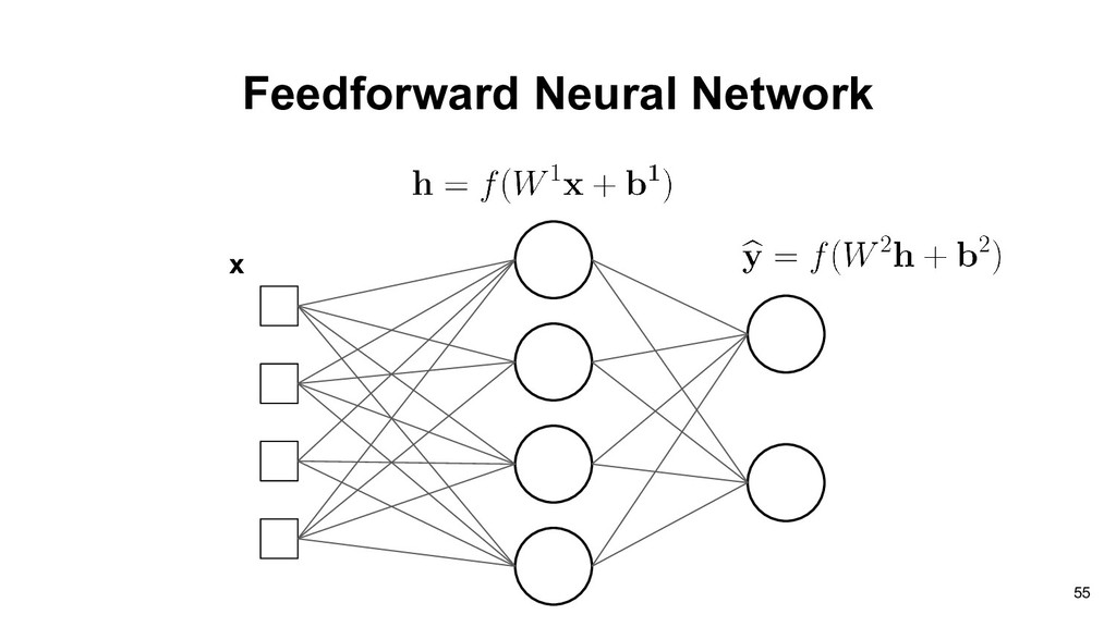
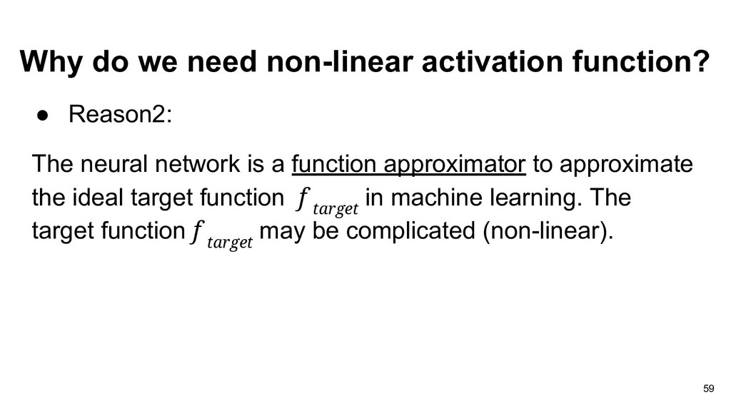
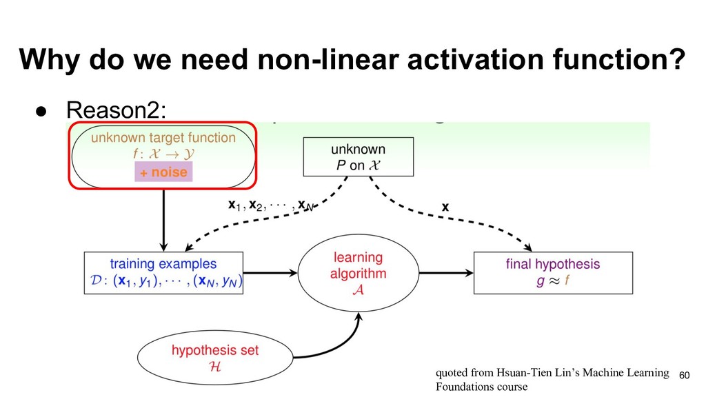
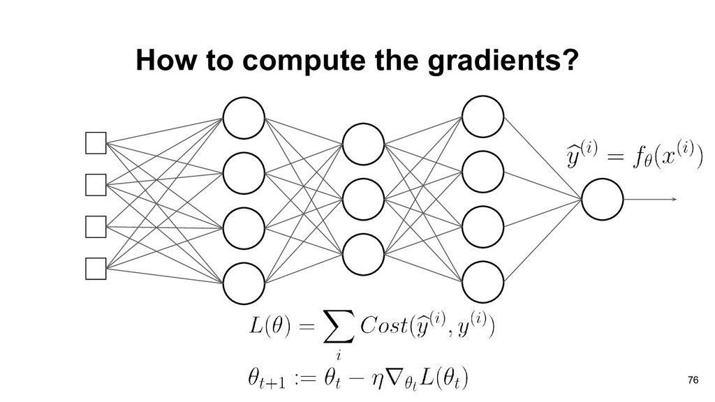
59. Why do we need non-linear activation function? • Reason2: The neural network is a function approximator to approximate the ideal target function f target in machine learning. The target function f target may be complicated (non-linear). 59
60. • Reason2: Why do we need non-linear activation function? quoted from Hsuan-Tien Lin’s Machine Learning Foundations course 60
61. From Linear to Non-Linear Use different kinds of activation function to transform the linear function to non-linear function. +1 0 +1 0 -1 The condition of linear function 61
62. Activation Function sigmoid function tanh function Relu function 62
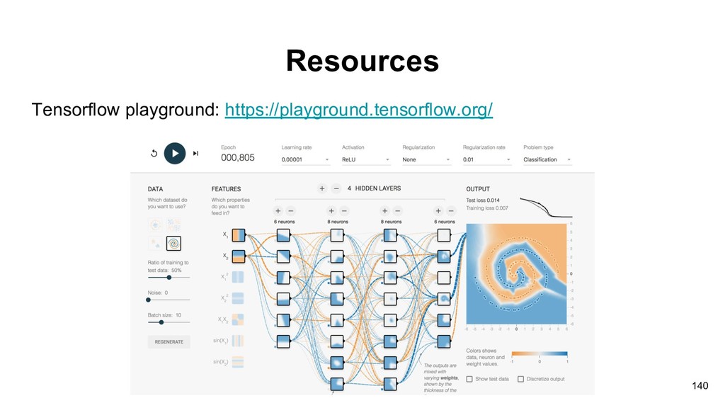
63. The decision boundary of Neural Network quoted from “Introductory Overview Lecture The Deep Learning Revolution” in JSM 2018 and you can play with ConvnetJS: https://cs.stanford.edu/people/karpathy/convnetjs/demo/classify2d.html 63
64. Thus, with non-linear transformation the neural network could be more powerful! 64
65. Model Capacity Deep Learning & Neural Network Multi-Layer Perceptron Linear Regression & Logistic Regression Model Capacity Low High 65
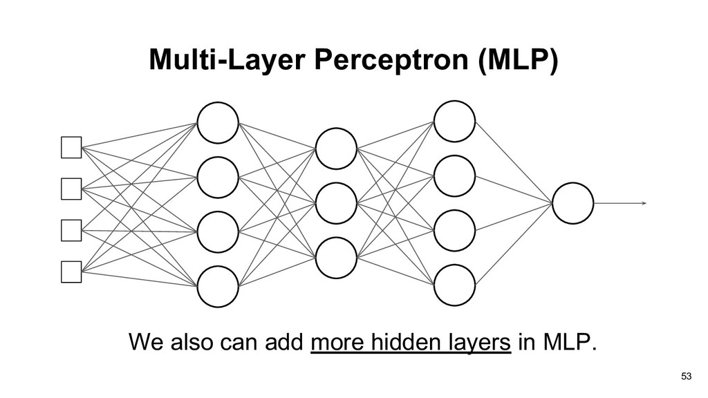
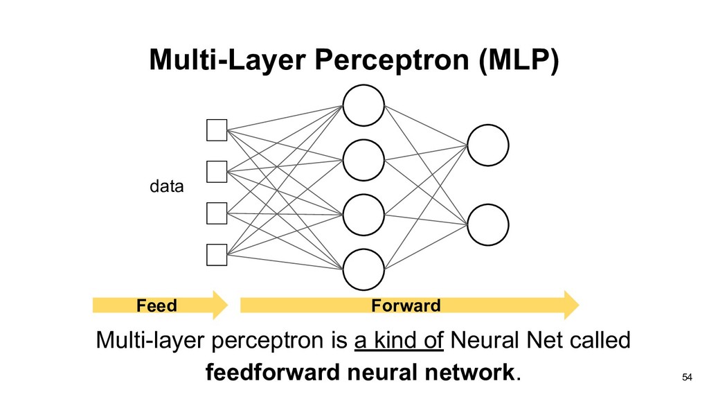
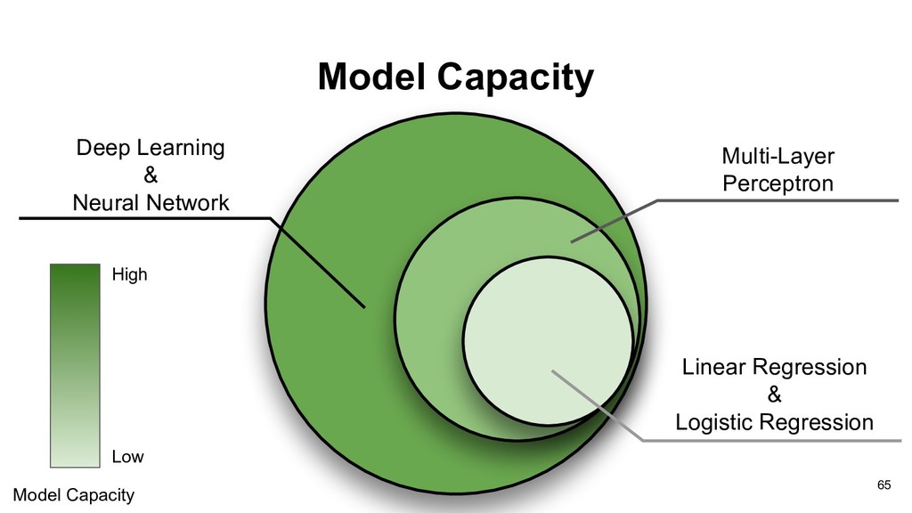
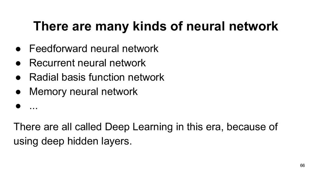
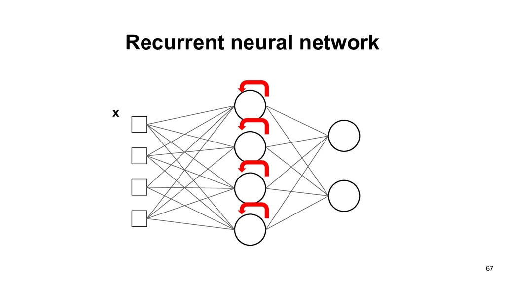
66. There are many kinds of neural network • Feedforward neural network • Recurrent neural network • Radial basis function network • Memory neural network • ... There are all called Deep Learning in this era, because of using deep hidden layers. 66
67. Recurrent neural network 67 x
68. What makes deep learning shine in many machine learning techniques? 68
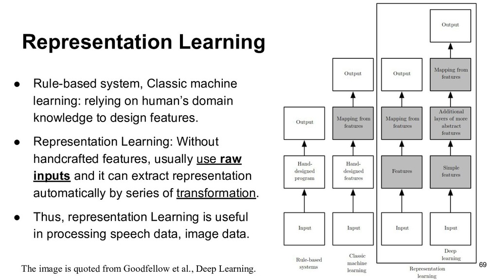
69. Representation Learning • Rule-based system, Classic machine learning: relying on human’s domain knowledge to design features. • Representation Learning: Without handcrafted features, usually use raw inputs and it can extract representation automatically by series of transformation. • Thus, representation Learning is useful in processing speech data, image data. The image is quoted from Goodfellow et al., Deep Learning. 69
70. Questions? 70
71. Learning in Neural Network Deep Learning is a subfield of machine learning, and we can learn the weights by optimization algorithm. Learning algorithms: • Gradient based method • Evolutionary method • ... 71
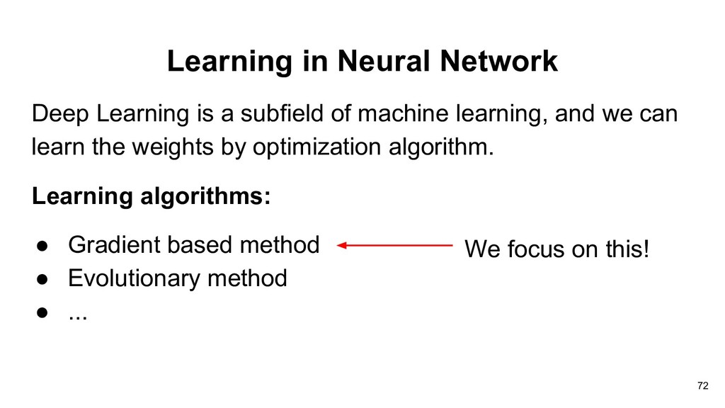
72. Learning in Neural Network Deep Learning is a subfield of machine learning, and we can learn the weights by optimization algorithm. Learning algorithms: • Gradient based method • Evolutionary method • ... We focus on this! 72
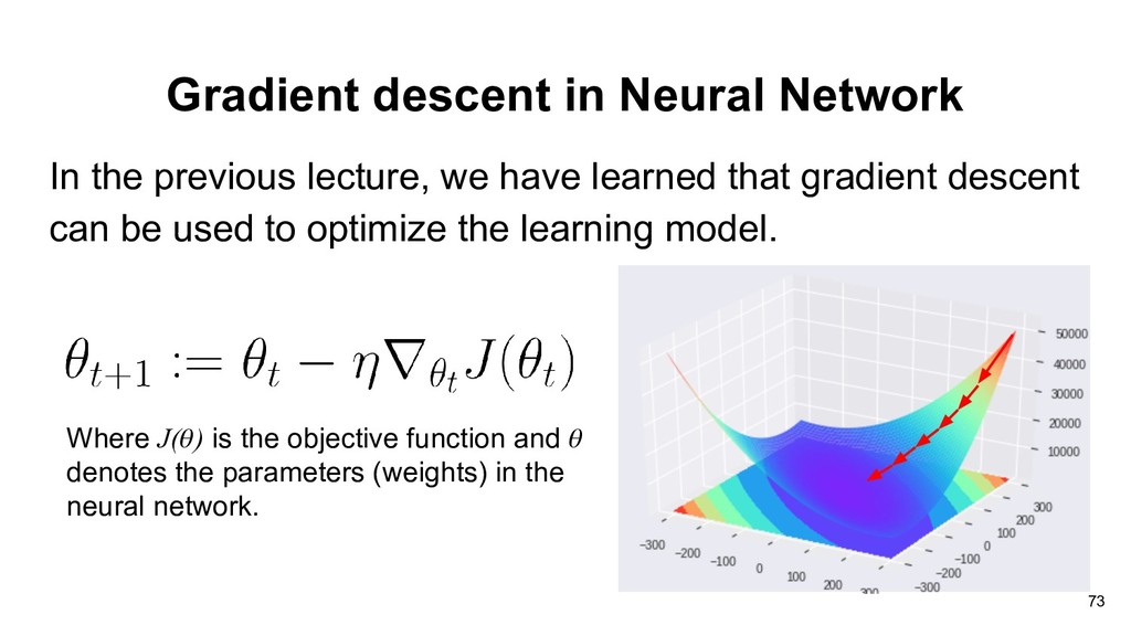
73. Gradient descent in Neural Network In the previous lecture, we have learned that gradient descent can be used to optimize the learning model. Where J( ) is the objective function and denotes the parameters (weights) in the neural network. 73
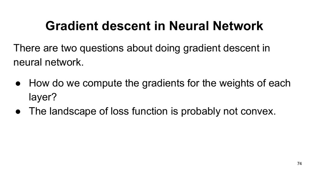
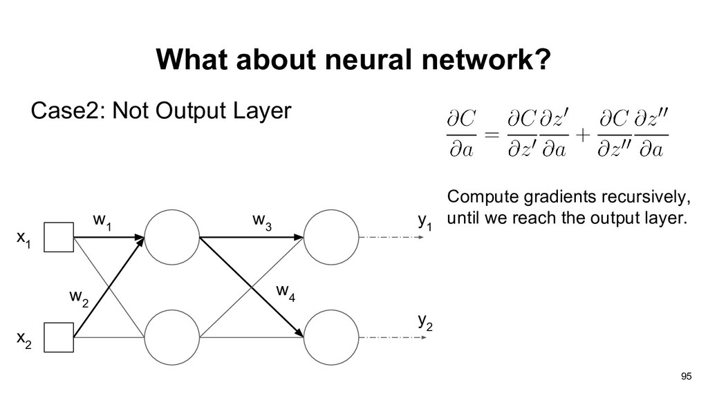
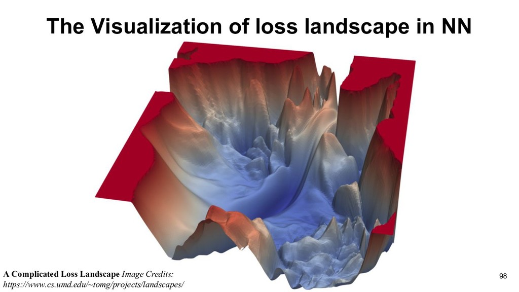
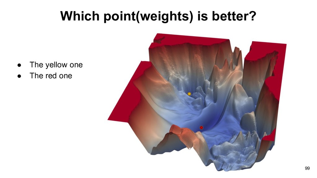
74. Gradient descent in Neural Network There are two questions about doing gradient descent in neural network. • How do we compute the gradients for the weights of each layer? • The landscape of loss function is probably not convex. 74
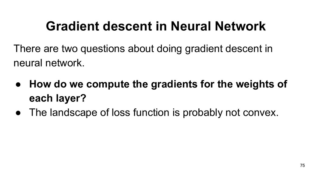
75. Gradient descent in Neural Network There are two questions about doing gradient descent in neural network. • How do we compute the gradients for the weights of each layer? • The landscape of loss function is probably not convex. 75
76. How to compute the gradients? 76
77. The operation in Neural Network Let’s think about the simplified example, there are 3 kinds of computation involves in neural network. • Addition • Multiplication • Activation x 1 w 1 x 2 w 2 b 77
78. A simplified example of backpropagation Consider a simple function f(x, y) = x + y. It can be expressed by a computational graph. ＋ x y z = f(x, y) = x + y 78
79. A simplified example of backpropagation Consider a simple function f(x, y) = xy. It can be expressed by a computational graph too. ＊ x y z = f(x, y) = xy 79
80. Consider the case of activation function: A simplified example of backpropagation f x z = f (x) 80
81. The derivative of activation function 81 sigmoid function tanh function Image Credits: http://ronny.rest/media/blog/2017/2017_08_16_tanh/tanh_v_sigmoid.jpg
82. The derivative of activation function 82 ReLU (Rectified Linear Unit)
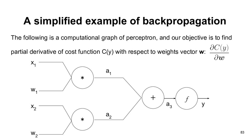
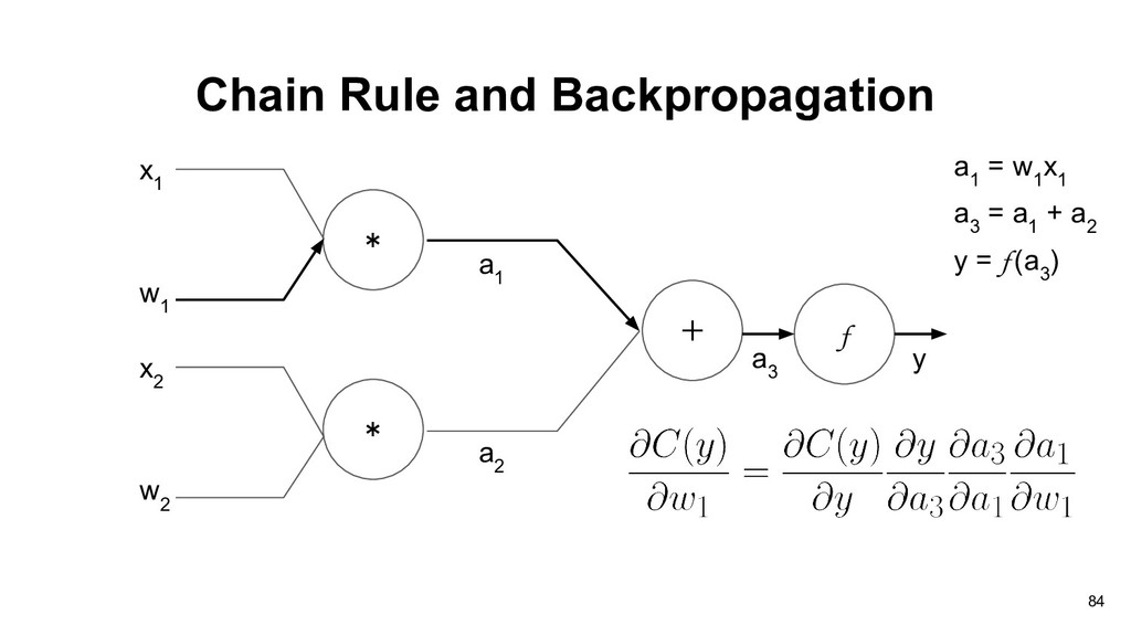
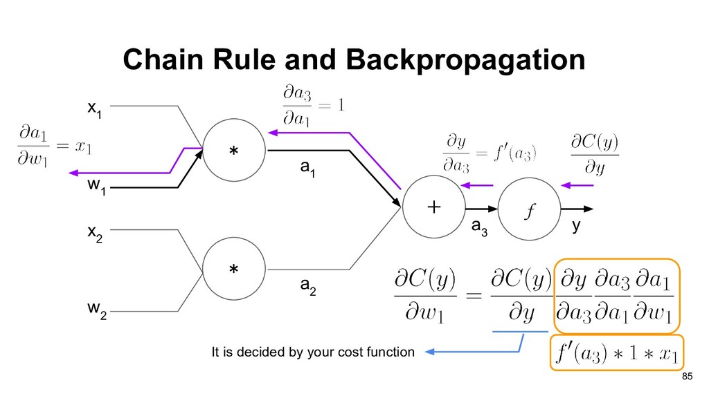
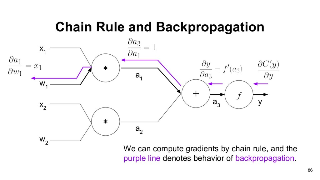
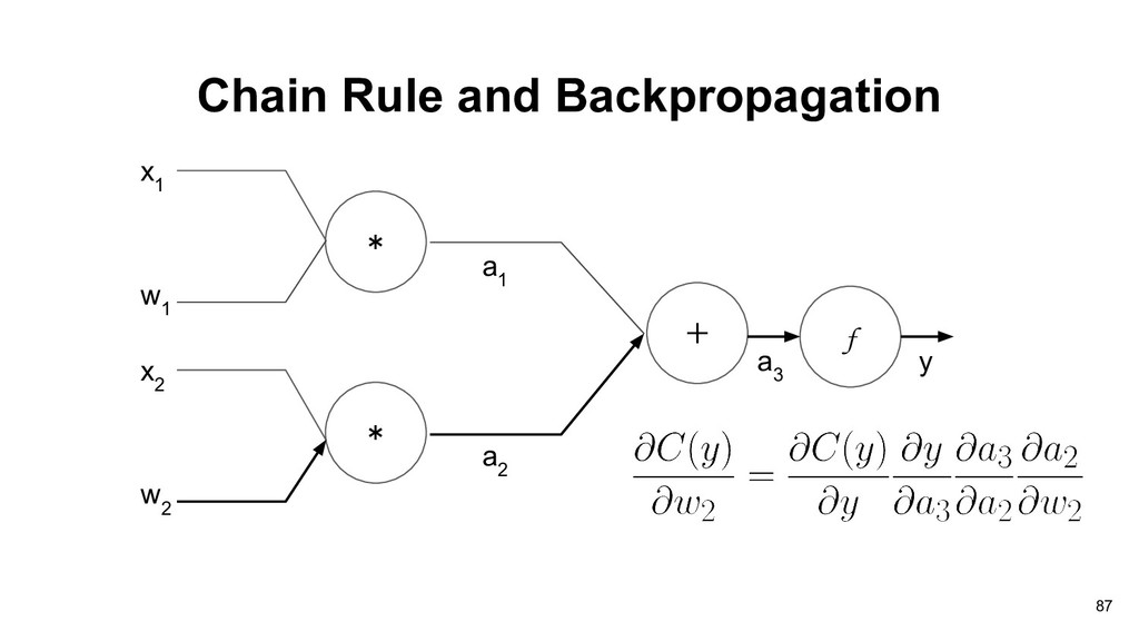
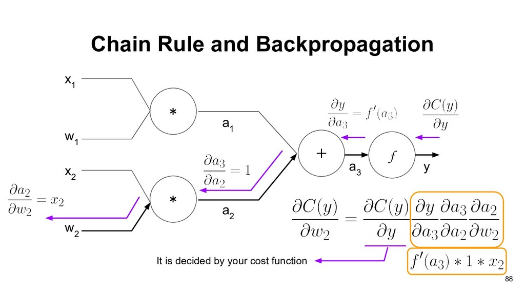
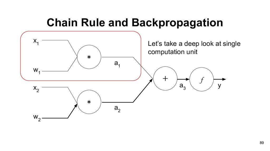
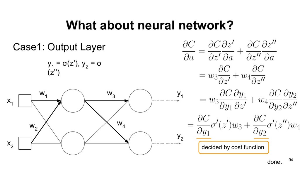
83. A simplified example of backpropagation The following is a computational graph of perceptron, and our objective is to find partial derivative of cost function C(y) with respect to weights vector w: ＊ ＊ x 1 ＋ w 1 x 2 w 2 a 1 a 2 f a 3 y 83
84. Chain Rule and Backpropagation ＊ ＊ x 1 ＋ w 1 x 2 w 2 a 2 f a 3 y 84 a 1 = w 1 x 1 a 3 = a 1 + a 2 y = f (a 3 ) a 1
85. Chain Rule and Backpropagation ＊ ＊ x 1 ＋ w 1 x 2 w 2 a 1 a 2 f a 3 y It is decided by your cost function 85
86. Chain Rule and Backpropagation ＊ ＊ x 1 ＋ w 1 x 2 w 2 a 1 a 2 f a 3 y We can compute gradients by chain rule, and the purple line denotes behavior of backpropagation. 86
87. Chain Rule and Backpropagation ＊ ＊ x 1 ＋ w 1 x 2 w 2 a 1 a 2 f a 3 y 87
88. Chain Rule and Backpropagation ＊ ＊ x 1 ＋ w 1 x 2 w 2 a 1 a 2 f a 3 y It is decided by your cost function 88
89. Chain Rule and Backpropagation ＊ ＊ x 1 ＋ w 1 x 2 w 2 a 1 a 2 f a 3 y Let’s take a deep look at single computation unit 89
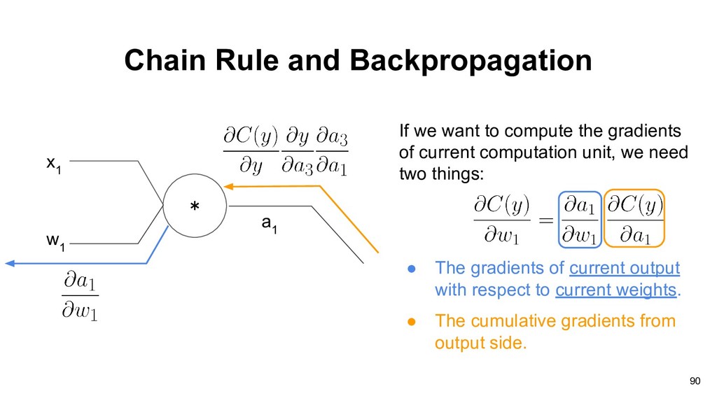
90. Chain Rule and Backpropagation ＊ x 1 w 1 a 1 If we want to compute the gradients of current computation unit, we need two things: • The gradients of current output with respect to current weights. • The cumulative gradients from output side. 90
91. What about neural network? We can consider each neuron in neural network a computation unit. x 1 x 2 Cost: C(θ) 91
92. What about neural network? Find: x 1 x 2 w 1 w 2 Cost: C(θ) w 3 w 4 92
93. What about neural network? Find: x 1 x 2 w 1 w 2 w 3 w 4 z = wTx + b a = σ(z) z’ = w 3 a + b 3 z’’ = w 4 a + b 4 93
94. What about neural network? Case1: Output Layer x 1 x 2 w 1 w 2 w 3 w 4 y 1 = σ(z’), y 2 = σ (z’’) y 1 y 2 done. decided by cost function 94
95. What about neural network? Case2: Not Output Layer x 1 x 2 w 1 w 2 w 3 w 4 y 1 y 2 Compute gradients recursively, until we reach the output layer. 95
96. Gradient descent in Neural Network There are two questions about doing gradient descent in neural network. • How do we compute the gradients for the weights of each layer? • The landscape of loss function is probably not convex. 96
97. Convex V.S Non-Convex 97 J(θ) θ θ J(θ) convex non-convex You can see math definition in wikipedia: https://en.wikipedia.org/wiki/Convex_function
98. The Visualization of loss landscape in NN A Complicated Loss Landscape Image Credits: https://www.cs.umd.edu/~tomg/projects/landscapes/ 98
99. Which point(weights) is better? • The yellow one • The red one 99
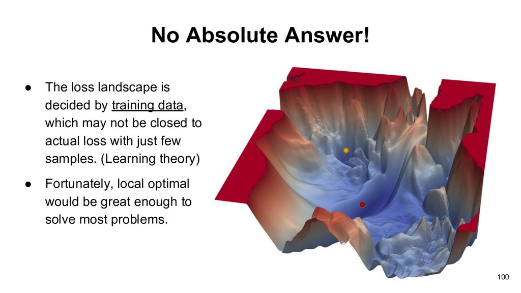
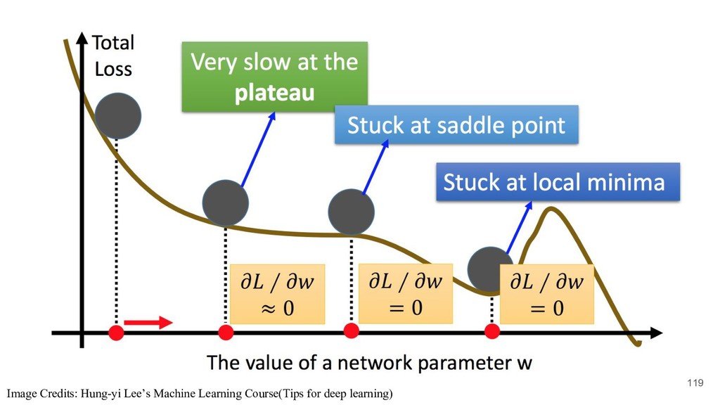
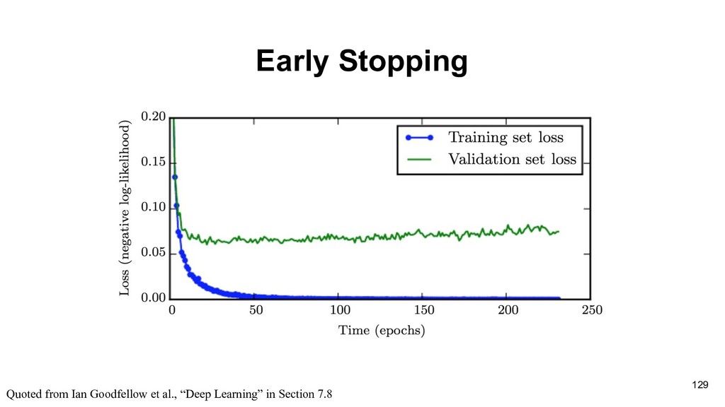
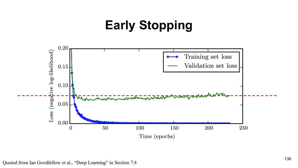
100. No Absolute Answer! • The loss landscape is decided by training data, which may not be closed to actual loss with just few samples. (Learning theory) • Fortunately, local optimal would be great enough to solve most problems. 100
101. The issues about gradient descent • Memory Usage • Vanishing gradients • Dying ReLUs • Exploding gradients in RNNs 101
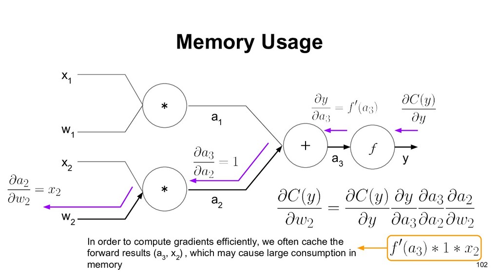
102. Memory Usage 102 ＊ ＊ x 1 ＋ w 1 x 2 w 2 a 1 a 2 f a 3 y In order to compute gradients efficiently, we often cache the forward results (a 3 , x 2 ) , which may cause large consumption in memory
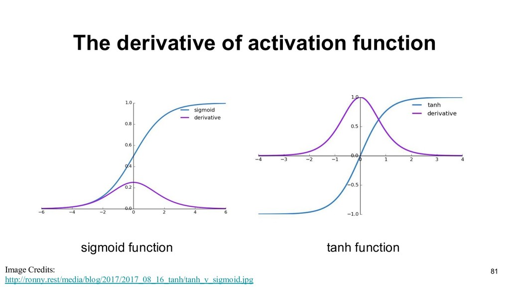
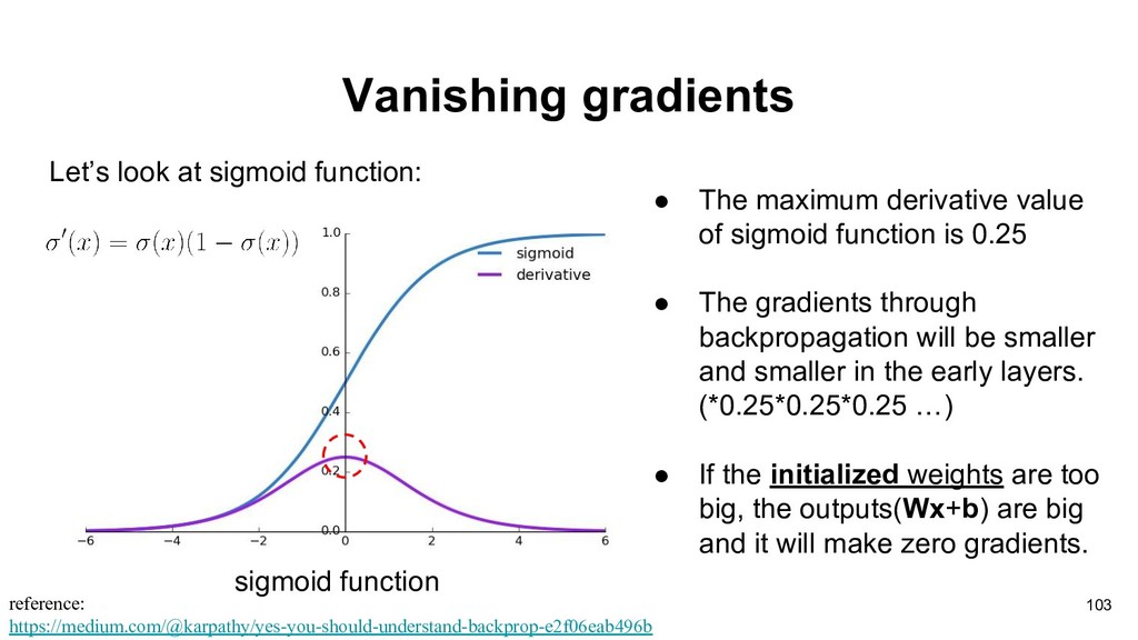
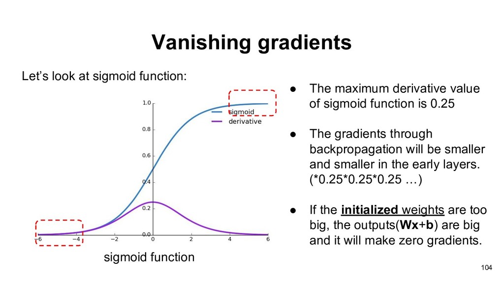
103. Vanishing gradients Let’s look at sigmoid function: 103 sigmoid function reference: https://medium.com/@karpathy/yes-you-should-understand-backprop-e2f06eab496b • The maximum derivative value of sigmoid function is 0.25 • The gradients through backpropagation will be smaller and smaller in the early layers. (*0.25*0.25*0.25 …) • If the initialized weights are too big, the outputs(Wx+b) are big and it will make zero gradients.
104. Vanishing gradients Let’s look at sigmoid function: 104 sigmoid function • The maximum derivative value of sigmoid function is 0.25 • The gradients through backpropagation will be smaller and smaller in the early layers. (*0.25*0.25*0.25 …) • If the initialized weights are too big, the outputs(Wx+b) are big and it will make zero gradients.
105. Vanishing gradients in tanh If we initialized large weights in neural network, it also makes vanishing gradients in tanh. 105
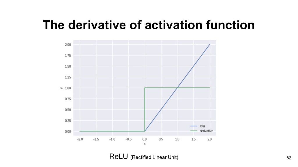
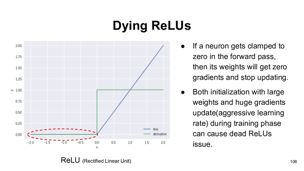
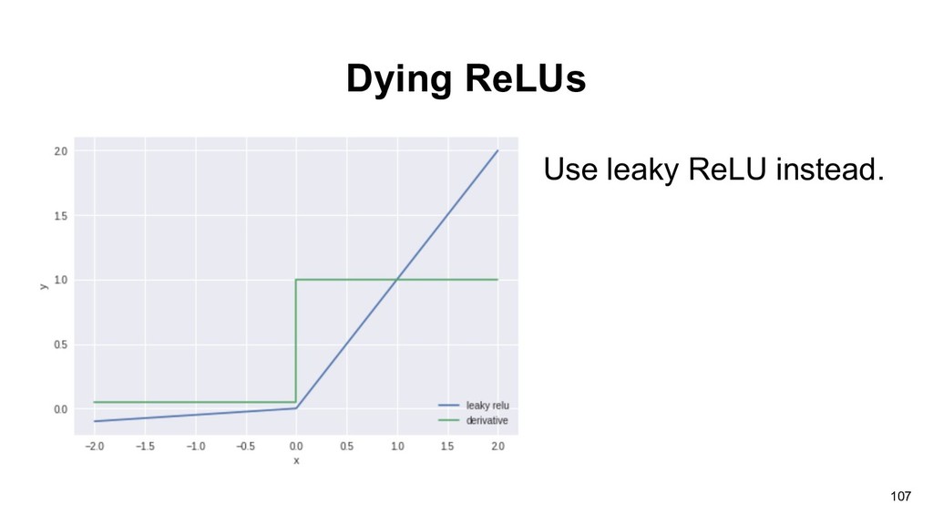
106. Dying ReLUs • If a neuron gets clamped to zero in the forward pass, then its weights will get zero gradients and stop updating. • Both initialization with large weights and huge gradients update(aggressive learning rate) during training phase can cause dead ReLUs issue. 106 ReLU (Rectified Linear Unit)
107. Dying ReLUs Use leaky ReLU instead. 107
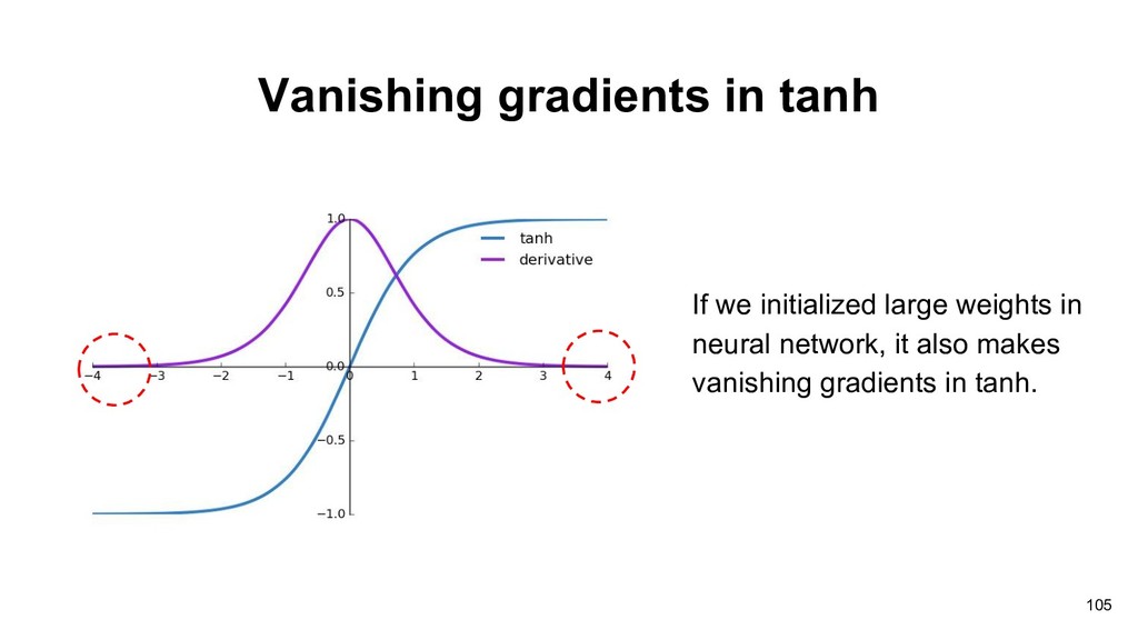
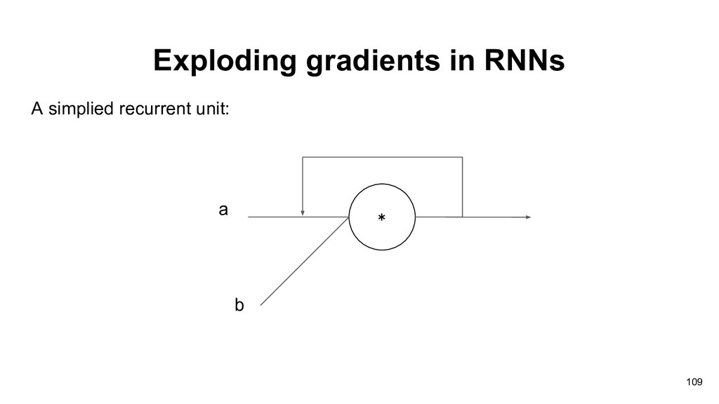
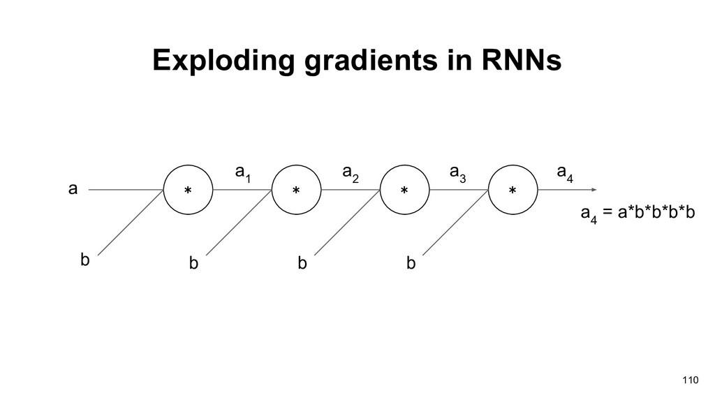
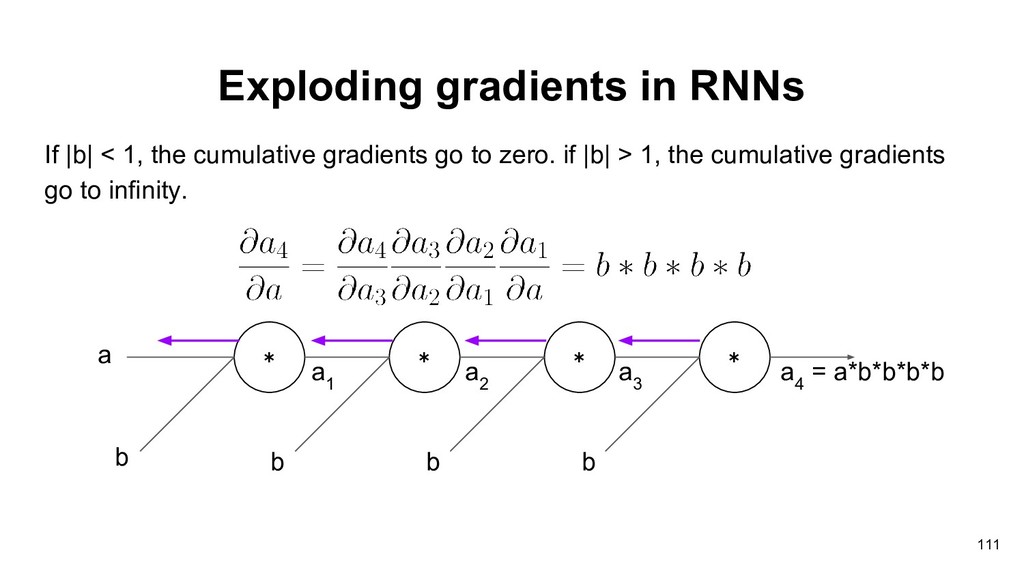
108. Exploding gradients in RNNs Sometimes, the gradients may explode, especially in vanilla recurrent neural network(原始的RNN). Pascanu et al. addressed this problem and proposed a solution called gradients clipping to relieve exploding gradients. A special recurrent unit LSTM can relieve this issue! 108 Pascanu et al., “On the difficulty of training Recurrent Neural Networks”
109. Exploding gradients in RNNs 109 ＊ a b A simplied recurrent unit:
110. Exploding gradients in RNNs 110 ＊ ＊ ＊ ＊ a b b b b a 4 = a*b*b*b*b a 1 a 2 a 3 a 4
111. Exploding gradients in RNNs If |b| < 1, the cumulative gradients go to zero. if |b| > 1, the cumulative gradients go to infinity. 111 ＊ ＊ ＊ ＊ a b b b b a 4 = a*b*b*b*b a 1 a 2 a 3
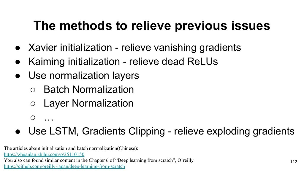
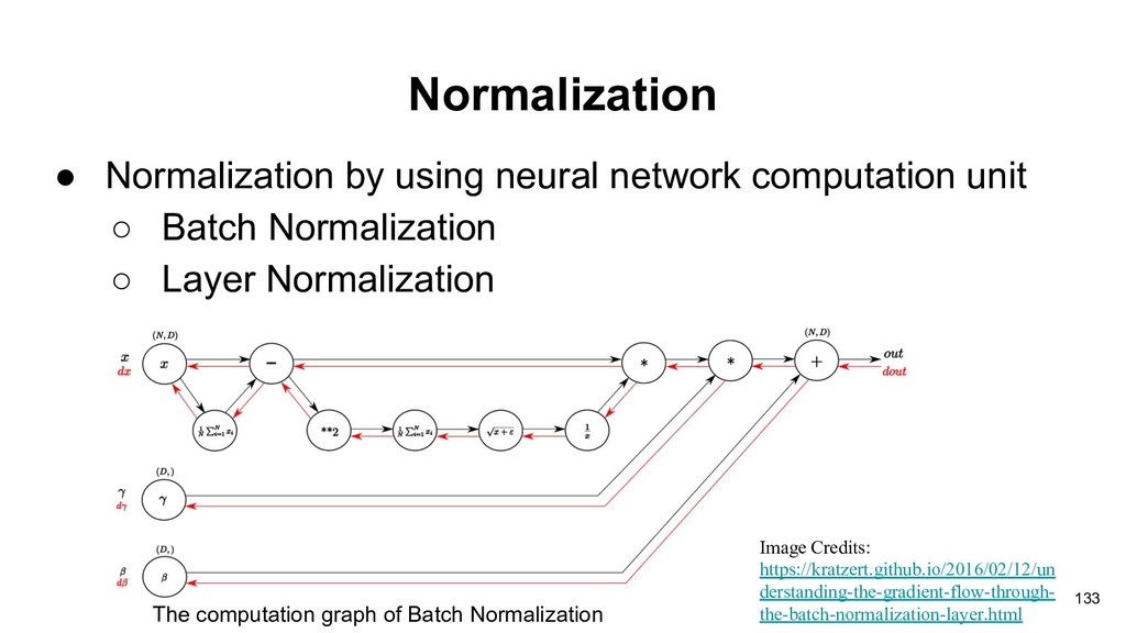
112. The methods to relieve previous issues • Xavier initialization - relieve vanishing gradients • Kaiming initialization - relieve dead ReLUs • Use normalization layers ◦ Batch Normalization ◦ Layer Normalization ◦ … • Use LSTM, Gradients Clipping - relieve exploding gradients 112 The articles about initialization and batch normalization(Chinese): https://zhuanlan.zhihu.com/p/25110150 You also can found similar content in the Chapter 6 of “Deep learning from scratch”, O’reilly https://github.com/oreilly-japan/deep-learning-from-scratch
113. The resources about backpropagation • Lecture notes of CS231n, Stanford ◦ http://cs231n.github.io/optimization-1/ • Hung-Yi Lee’s course video in NTU, Taiwan ◦ https://www.youtube.com/watch?v=ibJpTrp5mcE&list=PLJV_el3uVTsPy9oCRY30oBPNLCo89 yu49&index=12 • An article from Andrej Karpathy ◦ Yes you should understand backprop: https://medium.com/@karpathy/yes-you-should-understand-backprop-e2f06eab496b 113
114. Questions? 114
115. Tips for training deep neural network 115 • Choose Optimizer • Data augmentation • Regularization • Early Stopping • Normalization
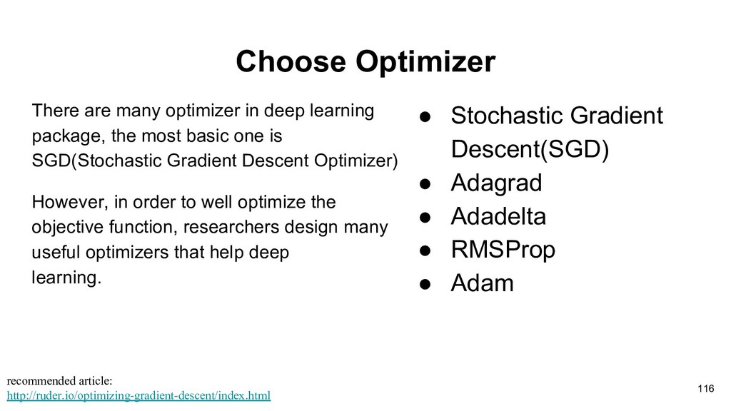
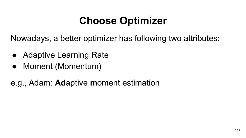
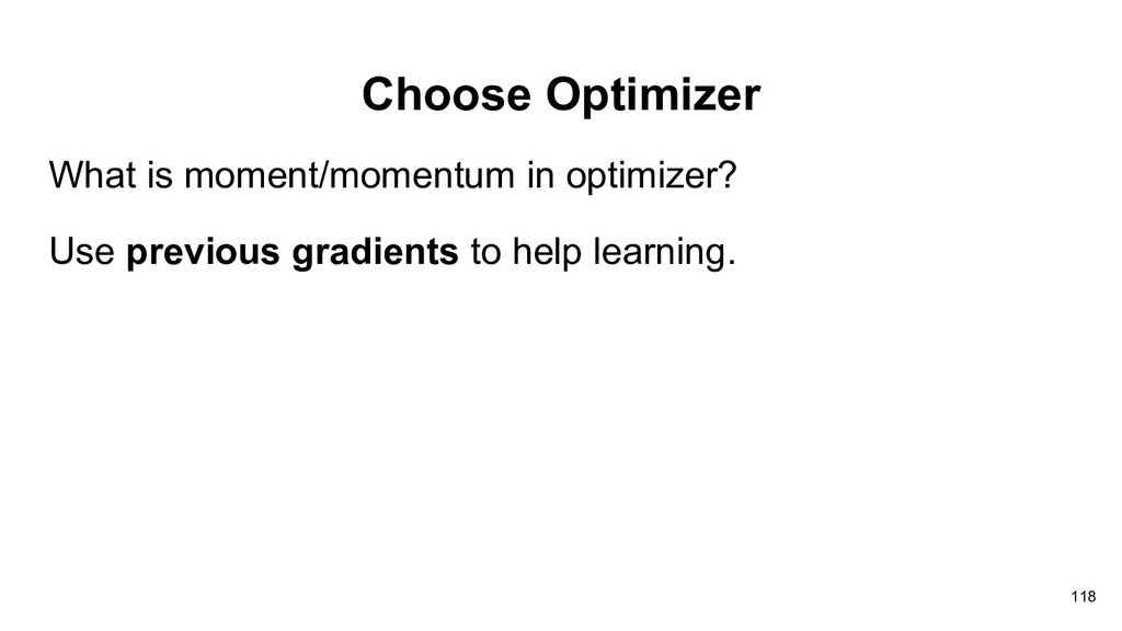
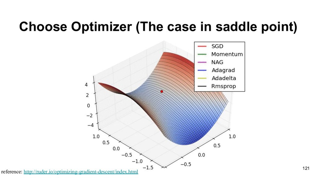
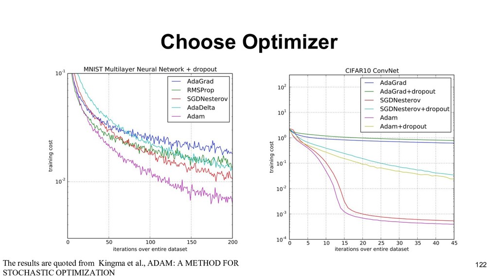
116. Choose Optimizer There are many optimizer in deep learning package, the most basic one is SGD(Stochastic Gradient Descent Optimizer) However, in order to well optimize the objective function, researchers design many useful optimizers that help deep learning.Improving Deep Neural Networks: Hyperparameter tuning, Regularization and Optimization 116 • Stochastic Gradient Descent(SGD) • Adagrad • Adadelta • RMSProp • Adam recommended article: http://ruder.io/optimizing-gradient-descent/index.html
117. Choose Optimizer Nowadays, a better optimizer has following two attributes: • Adaptive Learning Rate • Moment (Momentum) e.g., Adam: Adaptive moment estimation 117
118. Choose Optimizer What is moment/momentum in optimizer? Use previous gradients to help learning. 118
119. 119 Image Credits: Hung-yi Lee’s Machine Learning Course(Tips for deep learning)
120. 120 Image Credits: Hung-yi Lee’s Machine Learning Course(Tips for deep learning)
121. Choose Optimizer (The case in saddle point) 121 reference: http://ruder.io/optimizing-gradient-descent/index.html
122. Choose Optimizer 122 The results are quoted from Kingma et al., ADAM: A METHOD FOR STOCHASTIC OPTIMIZATION
123. Choose Adam in default. 123 reference: https://machinelearningmastery.com/adam-optimization-algorithm-for-deep-learning/
124. Data augmentation 124 Increase the generalizability of model(avoid overfitting) by giving additional human-modified data, including noise. (Image: rotation，scaling，panning，flipping，in different angle)
125. Data augmentation Be careful!! DO NOT apply transformations that would change the correct class. 125 Image from MNIST
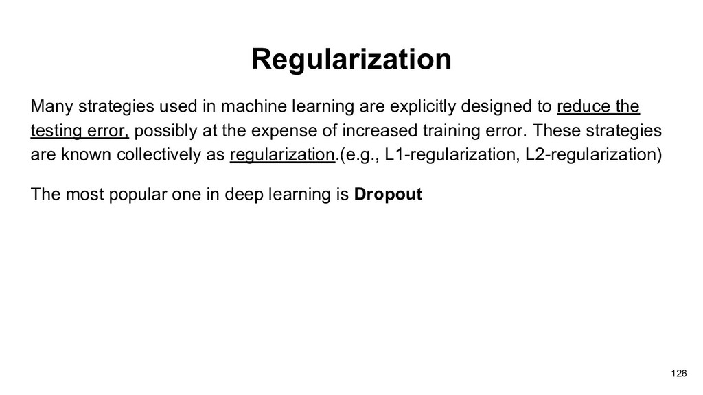
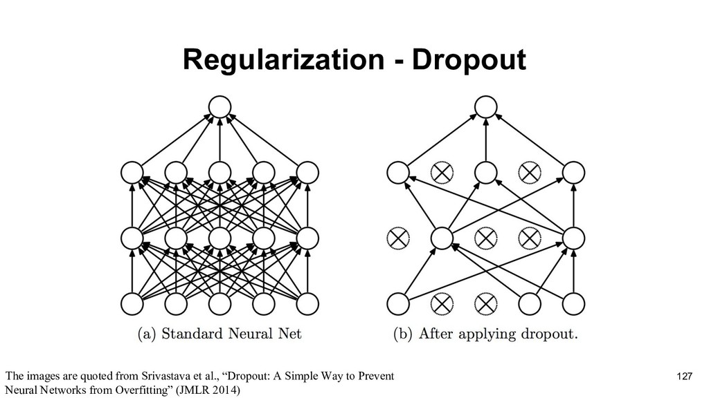
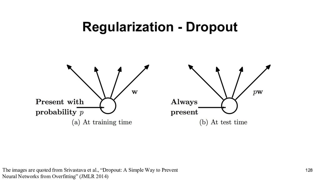
126. Regularization Many strategies used in machine learning are explicitly designed to reduce the testing error, possibly at the expense of increased training error. These strategies are known collectively as regularization.(e.g., L1-regularization, L2-regularization) The most popular one in deep learning is Dropout 126
127. Regularization - Dropout 127 The images are quoted from Srivastava et al., “Dropout: A Simple Way to Prevent Neural Networks from Overfitting” (JMLR 2014)
128. Regularization - Dropout 128 The images are quoted from Srivastava et al., “Dropout: A Simple Way to Prevent Neural Networks from Overfitting” (JMLR 2014)
129. Early Stopping 129 Quoted from Ian Goodfellow et al., “Deep Learning” in Section 7.8
130. Early Stopping 130 Quoted from Ian Goodfellow et al., “Deep Learning” in Section 7.8
131. Normalization • Handcrafted Data Normalization • Normalization by using neural network computation unit 131
132. Normalization 132 This slide was borrowed from Andrew Ng’s Machine Learning Course
133. Normalization • Normalization by using neural network computation unit ◦ Batch Normalization ◦ Layer Normalization 133 The computation graph of Batch Normalization Image Credits: https://kratzert.github.io/2016/02/12/un derstanding-the-gradient-flow-through- the-batch-normalization-layer.html
134. Normalization • Normalization by using neural network computation unit ◦ Batch Normalization ◦ Layer Normalization Notice!! The behavior of normalization layer may be different in training and testing. 134
135. Resources about CNN CNN, Convolutional Neural Network. CNN is popular neural network architecture in deep learning, especially in computer vision tasks. Here are some nice resources: • CS231n, Stanford: http://cs231n.stanford.edu/ • ConvNetJS: https://cs.stanford.edu/people/karpathy/convnetjs/index.html • Article: An Intuitive Explanation of Convolutional Neural Networks: https://ujjwalkarn.me/2016/08/11/intuitive-explanation-convnets/ • Intuitively Understanding Convolutions for Deep Learning: https://towardsdatascience.com/intuitively-understanding-convolutions-for-deep-learning-1f6f42faee 1 • Intuitively Understanding Convolutions for Deep Learning (Chinese) http://bangqu.com/nNMB58.html#utm_source=Facebook_PicSee&utm_medium=Social 135
136. Implementation 136
137. Pytorch Installation on Google Colab 137 https://gist.github.com/JIElite/2a0643cb256cc96517ad1cbc2280dbf8
138. Reference Book • Deep Learning • Neural Network Design • Learning from Data Course • CS229, Stanford • CS231n, Stanford • Hsuan-Tien Lin’s Machine Learning Foundations, National Taiwan University • Hung-yi Lee’s Machine Learning, National Taiwan University And some papers and articles 138
139. Resources • Deep Learning(Nature): ◦ https://www.evl.uic.edu/creativecoding/courses/cs523/slides/week3/Deep Learning_LeCun.pdf • Pytorch examples: ◦ https://github.com/jcjohnson/pytorch-examples • CS230 code example: ◦ https://github.com/cs230-stanford/cs230-code-examples • Introductory Overview Lecture The Deep Learning Revolution: ◦ http://www.cs.cmu.edu/~rsalakhu/jsm2018.html • Why softmax is named “soft”max? ◦ http://neuralnetworksanddeeplearning.com/chap3.html#softmax 139
140. Resources Tensorflow playground: https://playground.tensorflow.org/ 140