Regularization and Representer Theorems

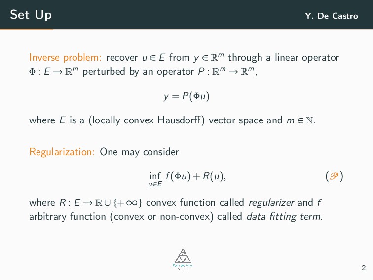
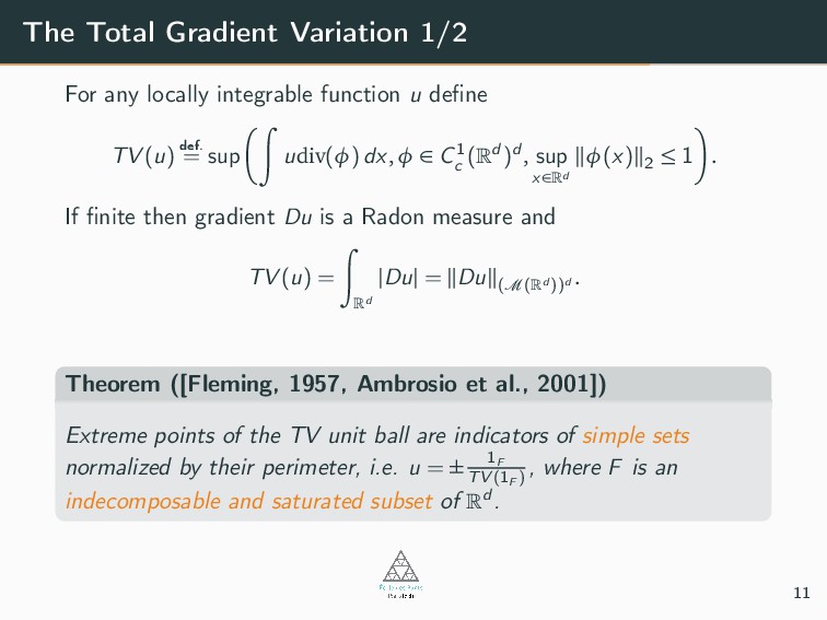
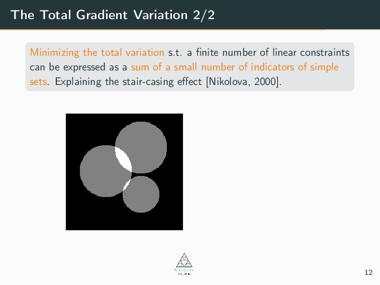
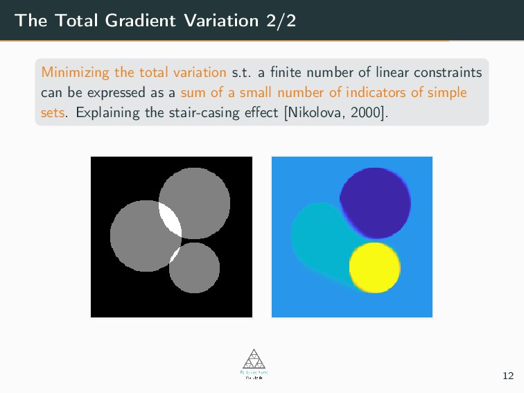
We establish a general principle which states that regularizing an inverse problem with a convex function yields solutions which are convex combinations of a small number of atoms. These atoms are identified with the extreme points and elements of the extreme rays of the regularizer level sets. An extension to a broader class of quasi-convex regularizers is also discussed. As a side result, we characterize the minimizers of the total gradient variation, which was still an unresolved problem.

Transcript

1. Regularization and Representer Theorems on a topology-free diet Yohann De Castro (CERMICS) Labex Day, 4th December 2018
2. C. Boyer A. Chambolle V. Duval F. de Gournay P. Weiss 0
3. Outline Y. De Castro 1. Inverse Problems Regularization 2. Lineality Space, Extreme Rays 3. A Representer Theorem 4. Examples of Applications 1
4. Inverse Problems Regularization
5. Set Up Y. De Castro Inverse problem: recover u ∈ E from y ∈ m through a linear operator Φ : E → m perturbed by an operator P : m → m, y = P(Φu) where E is a (locally convex Hausdorff) vector space and m ∈ . 2
6. Set Up Y. De Castro Inverse problem: recover u ∈ E from y ∈ m through a linear operator Φ : E → m perturbed by an operator P : m → m, y = P(Φu) where E is a (locally convex Hausdorff) vector space and m ∈ . Regularization: One may consider inf u∈E f (Φu) + R(u), ( ) where R : E → ∪ {+∞} convex function called regularizer and f arbitrary function (convex or non-convex) called data fitting term. 2
7. Representer of Tikhonov regularization Y. De Castro One can be interested in [Scholkopf and Smola, 2001] min u∈ m 1 2 Φu − y 2 2 + 1 2 Lu 2 2 , where Φ ∈ m×n, L ∈ p×n s.t. kerΦ ∩ kerL = {0}. 3
8. Representer of Tikhonov regularization Y. De Castro One can be interested in [Scholkopf and Smola, 2001] min u∈ m 1 2 Φu − y 2 2 + 1 2 Lu 2 2 , where Φ ∈ m×n, L ∈ p×n s.t. kerΦ ∩ kerL = {0}. Solutions are u = m i=1 αi ψi + uK , with uK ∈ ker(L) and ψi = (Φ Φ + L L)−1(φi ) denoting φ i ∈ n the i-th row of Φ. 3
9. Lineality Space, Extreme Rays
10. Linearly Closed, Recession Cone and Lineality Space Let E be a real vector space and let C ⊆ E be a convex set. Linearly Closed (resp. linearly bounded) as "Topology-free" Diet Any intersection of C and a line of E is closed (resp. bounded) for the natural topology of the line. 4
11. Linearly Closed, Recession Cone and Lineality Space Let E be a real vector space and let C ⊆ E be a convex set. Linearly Closed (resp. linearly bounded) as "Topology-free" Diet Any intersection of C and a line of E is closed (resp. bounded) for the natural topology of the line. Recession Cone, rec(C) Set of all v ∈ E s.t. C + ∗ + v ⊆ C. It is a convex cone. 4
12. Linearly Closed, Recession Cone and Lineality Space Let E be a real vector space and let C ⊆ E be a convex set. Linearly Closed (resp. linearly bounded) as "Topology-free" Diet Any intersection of C and a line of E is closed (resp. bounded) for the natural topology of the line. Recession Cone, rec(C) Set of all v ∈ E s.t. C + ∗ + v ⊆ C. It is a convex cone. Lineality Space, lin(C) lin(C) := rec(C) ∩ (−rec(C)) 4
13. Extreme points and Extreme Rays Extreme Points and Rays Extreme Points: points p ∈ C s.t. C \ {p} is convex; 5
14. Extreme points and Extreme Rays Extreme Points and Rays Extreme Points: points p ∈ C s.t. C \ {p} is convex; Extreme Rays: rays ρ ∈ C s.t. if x,y ∈ C and ]x,y[ intersects ρ, then ]x,y[⊂ ρ; 5
15. Extreme points and Extreme Rays Extreme Points and Rays Extreme Points: points p ∈ C s.t. C \ {p} is convex; Extreme Rays: rays ρ ∈ C s.t. if x,y ∈ C and ]x,y[ intersects ρ, then ]x,y[⊂ ρ; Faces C (p): Union of {p} and all the open segments in C which have p as an inner point; 5
16. Extreme points and Extreme Rays Extreme Points and Rays Extreme Points: points p ∈ C s.t. C \ {p} is convex; Extreme Rays: rays ρ ∈ C s.t. if x,y ∈ C and ]x,y[ intersects ρ, then ]x,y[⊂ ρ; Faces C (p): Union of {p} and all the open segments in C which have p as an inner point; Faces description and Quotienting by lines Denote W a supplement of lin(C) and C := C ∩ W then C = C + lin(C), and { C (p) + lin(C)}p∈C = { C (p)}p∈C is the partition of C in elementary faces. 5
17. A Representer Theorem
18. Representer Theorem Denote t the optimal value of (1) given by min u∈E R(u) s.t. Φu = y , (1) its solution set, and C def. = u ∈ E : R(u) ≤ t . 6
19. Representer Theorem Denote t the optimal value of (1) given by min u∈E R(u) s.t. Φu = y , (1) its solution set, and C def. = u ∈ E : R(u) ≤ t . Theorem ([Boyer et al., 2018]) If infE R < t < +∞, nonempty, C is linearly closed and contains no line, and p ∈ s.t. j is the dimension of the face (p). Then p belongs to a face of C with dimension at most m + j − 1 and it can be written as a convex combination of m + j extreme points of C , or m + j − 1 points of C , each an extreme point of C or in an extreme ray of C . 6
20. On a figure ρ1 ρ2 e0 e1 e2 Φ−1({y}) C Figure 1: For m = 2 with = C ∩ Φ−1({y}) made of an extreme point and an extreme ray. The extreme point is a convex combination of {e0 ,e1 }. Depending on their position, the points in the ray are a convex combination of {e0 ,e1 ,e2 } or a pair of points, one in ρ1 and the other in ρ2 . 7
21. Quotienting by lines on a figure E/K C Φ−1({y}) ˜ C q1 q2 K = lin(C ) Figure 2: Quotienting by K = lin(C ) yields a level set C with no line. 8
22. Quotienting by lines on a figure E/K C Φ−1({y}) ˜ C q1 q2 K = lin(C ) Figure 2: Quotienting by K = lin(C ) yields a level set C with no line. With ˜ q1 ,..., ˜ qr ∈ ˜ C , d def. = dimΦ(K), r ≤ m + j − d (−1), p = r i=1 θi ψ−1 K (˜ qi ,0) qi ∈E +uK , where θi ≥ 0, r i=1 θi = 1, and uK ∈ K. 8
23. Examples of Applications
24. Linear Programming and the Moment Problem inf µ∈ + (Ω) Φµ=y 〈ψ,u〉. (2) with Ω compact metric space, + (Ω) nonnegative Radon measures, ψ and (φi )1≤i≤m continuous. 9
25. Linear Programming and the Moment Problem inf µ∈ + (Ω) Φµ=y 〈ψ,u〉. (2) with Ω compact metric space, + (Ω) nonnegative Radon measures, ψ and (φi )1≤i≤m continuous. Assume that the solution set (2) is nonempty. Then, its extreme points are m-sparse, i.e. of the form: u = m i=1 αi δxi , xi ∈ Ω,αi ≥ 0. 9
26. The Total Variation ball B = u ∈ (Ω) : u ≤ 1 with Ω open subset of d and (Ω) Radon measures. One has ext(B ) = {±δx , x ∈ Ω} 10
27. The Total Variation ball B = u ∈ (Ω) : u ≤ 1 with Ω open subset of d and (Ω) Radon measures. One has ext(B ) = {±δx , x ∈ Ω} Total variation regularized problems of the form: inf u∈ f (Φu) + u , yield m-sparse solutions (under an existence assumption). 10
28. The Total Gradient Variation 1/2 For any locally integrable function u define TV (u) def. = sup udiv(φ)dx,φ ∈ C1 c ( d )d , sup x∈ d φ(x) 2 ≤ 1 . If finite then gradient Du is a Radon measure and TV (u) = d |Du| = Du ( ( d ))d . 11
29. The Total Gradient Variation 1/2 For any locally integrable function u define TV (u) def. = sup udiv(φ)dx,φ ∈ C1 c ( d )d , sup x∈ d φ(x) 2 ≤ 1 . If finite then gradient Du is a Radon measure and TV (u) = d |Du| = Du ( ( d ))d . Theorem ([Fleming, 1957, Ambrosio et al., 2001]) Extreme points of the TV unit ball are indicators of simple sets normalized by their perimeter, i.e. u = ± 1F TV (1F ) , where F is an indecomposable and saturated subset of d . 11
30. The Total Gradient Variation 2/2 Minimizing the total variation s.t. a finite number of linear constraints can be expressed as a sum of a small number of indicators of simple sets. Explaining the stair-casing effect [Nikolova, 2000]. 12
31. The Total Gradient Variation 2/2 Minimizing the total variation s.t. a finite number of linear constraints can be expressed as a sum of a small number of indicators of simple sets. Explaining the stair-casing effect [Nikolova, 2000]. 12
32. References i Ambrosio, L., Caselles, V., Masnou, S., and Morel, J.-M. (2001). Connected components of sets of finite perimeter and applications to image processing. Journal of the European Mathematical Society, 3(1):39–92. Boyer, C., Chambolle, A., De Castro, Y., Duval, V., De Gournay, F., and Weiss, P. (2018). On representer theorems and convex regularization. arXiv preprint arXiv:1806.09810. Fleming, W. (1957). Functions with generalized gradient and generalized surfaces. Annali di Matematica Pura ed Applicata, 44(1):93–103. 13
33. References ii Nikolova, M. (2000). Local strong homogeneity of a regularized estimator. SIAM Journal on Applied Mathematics, 61(2):633–658. Scholkopf, B. and Smola, A. J. (2001). Learning with kernels: support vector machines, regularization, optimization, and beyond. MIT press. 14
34. Questions? 14