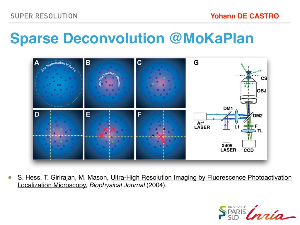
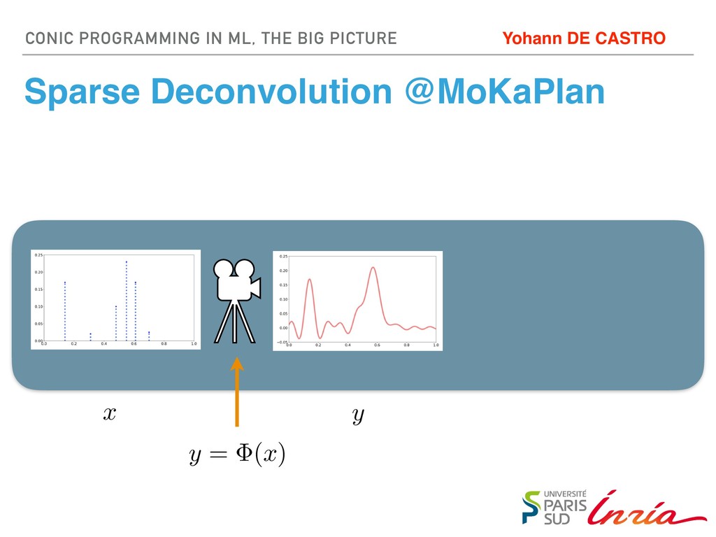
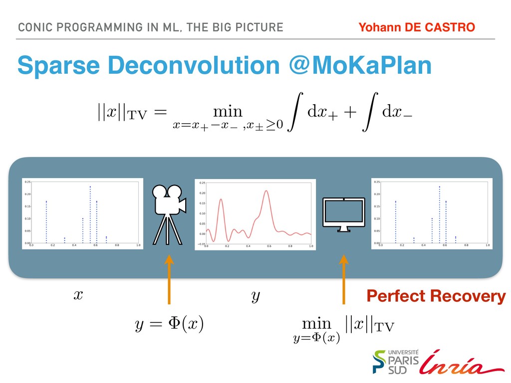
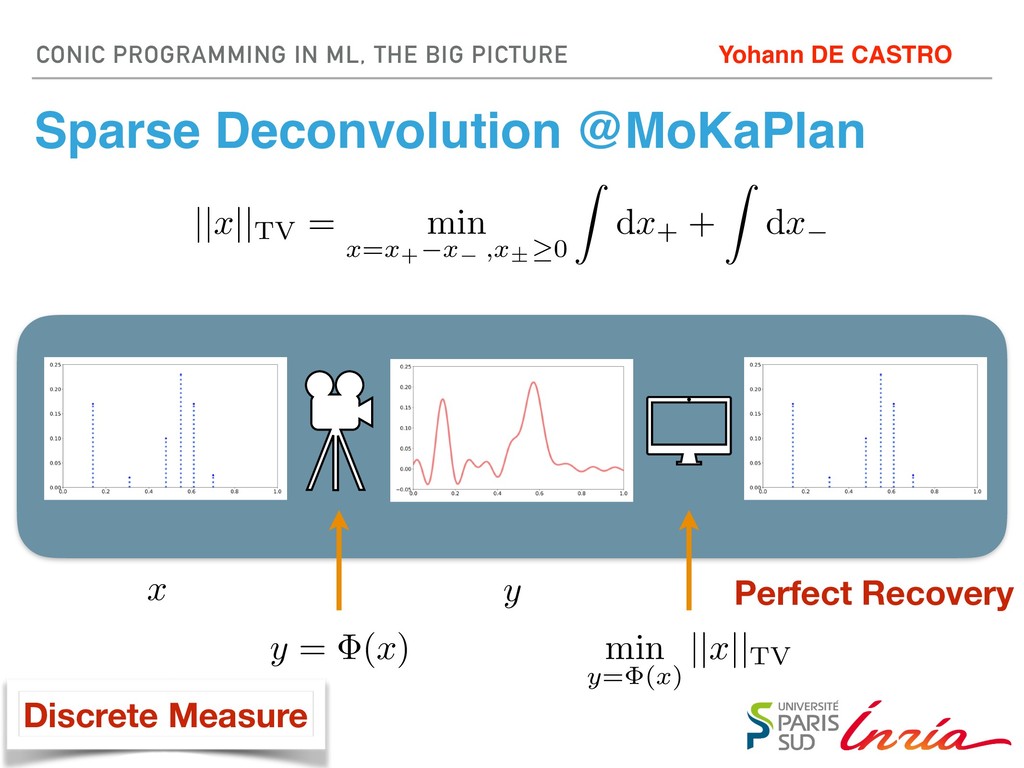
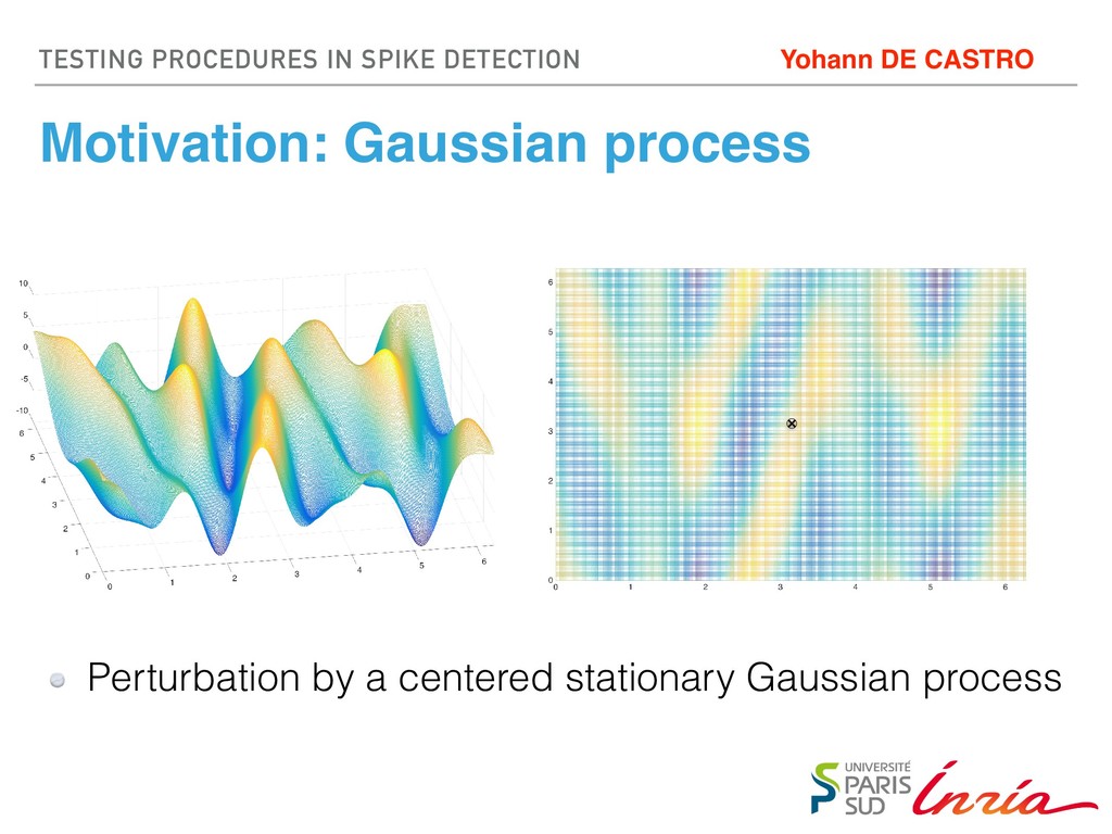
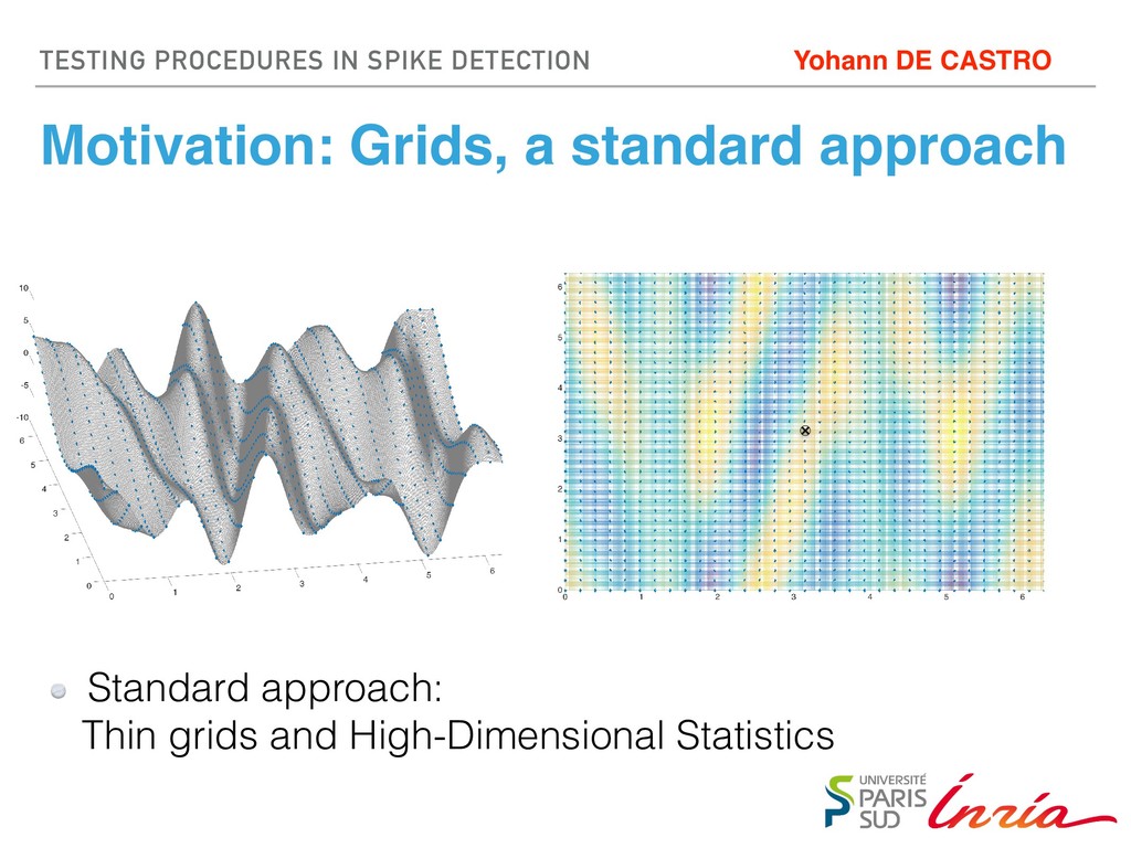
photoactivation and photobleaching, even if the density of fluorophore-labeled molecules is much higher than one fluorophore per mm2. We present a novel method by which fluorescence micros- copy may be performed to obtain an image with greatly enhanced ability to resolve large numbers of fluorescent 1. The spontaneous interconversion activated (fluorescent) state mus light-controlled activation rate. 2. For irreversible photoactivatio quantum yield must be finite a FIGURE 1 localization area contain (here, PA- neously wit for readout spatial illum a second on diode laser, Within the vation beam blue circles circles) and time, the ac (red Xs) an (black circl then activated, localized, and bleached until a sufficient number of molecules have been analyzed to construct an image. (G) Th the 405-nm activation laser (X405), which is reflected by a dichroic (DM1) to make it collinear with the Ar1 readout laser. A inverted fluorescence microscope is used to focus the lasers, which are reflected upward by a second dichroic mirror (DM2 objective lens (OBJ). The sample, supported by a coverslip (CS), emits fluorescence which is collected by the objective, transm and focused by the tube lens (TL) to form an image on a camera (CCD). Biophysica S. Hess, T. Girirajan, M. Mason, Ultra-High Resolution Imaging by Fluorescence Photoactivation Localization Microscopy, Biophysical Journal (2004). SUPER RESOLUTION
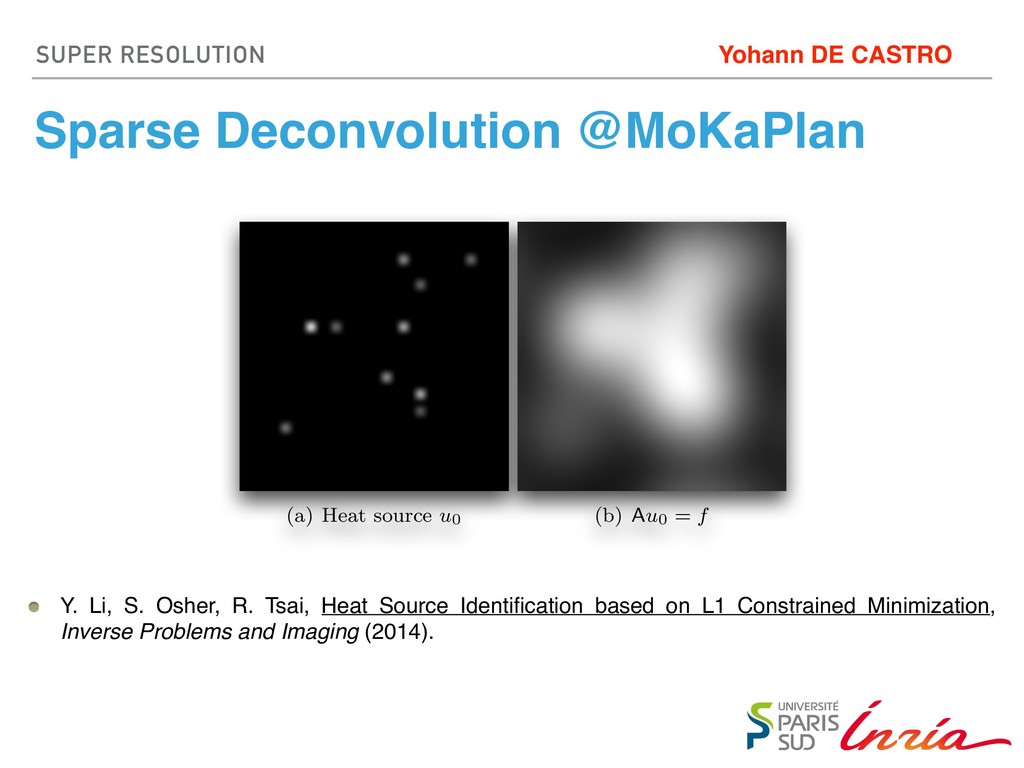
R. Tsai, Heat Source Identification based on L1 Constrained Minimization, Inverse Problems and Imaging (2014). 210 Yingying Li, Stanley Osher and Richard Tsai (a) Heat source u0 (b) Au0 = f (c) f + noise SUPER RESOLUTION
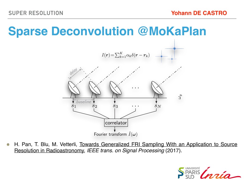
M. Vetterli, Towards Generalized FRI Sampling With an Application to Source Resolution in Radioastronomy, IEEE trans. on Signal Processing (2017). EE, Thierry Blu, Fellow, IEEE, and Martin Vetterli, Fellow, IEEE continuous-time arrival problem, rliest occurrence Prony’s method. n high resolution -time sparse sig- sampling theory ectral estimation pling. But not all fied by a concrete s, we develop the , typically sum of his by identifying uniform samples uniform samples A valid solution ization such that en measurements Fig. 1. Schematic diagram of a radio interferometer. The cross-corre of the received signals at different antennas are related to the Fourier tra of the sky image (see Table I) at certain non-uniform frequencies. SUPER RESOLUTION
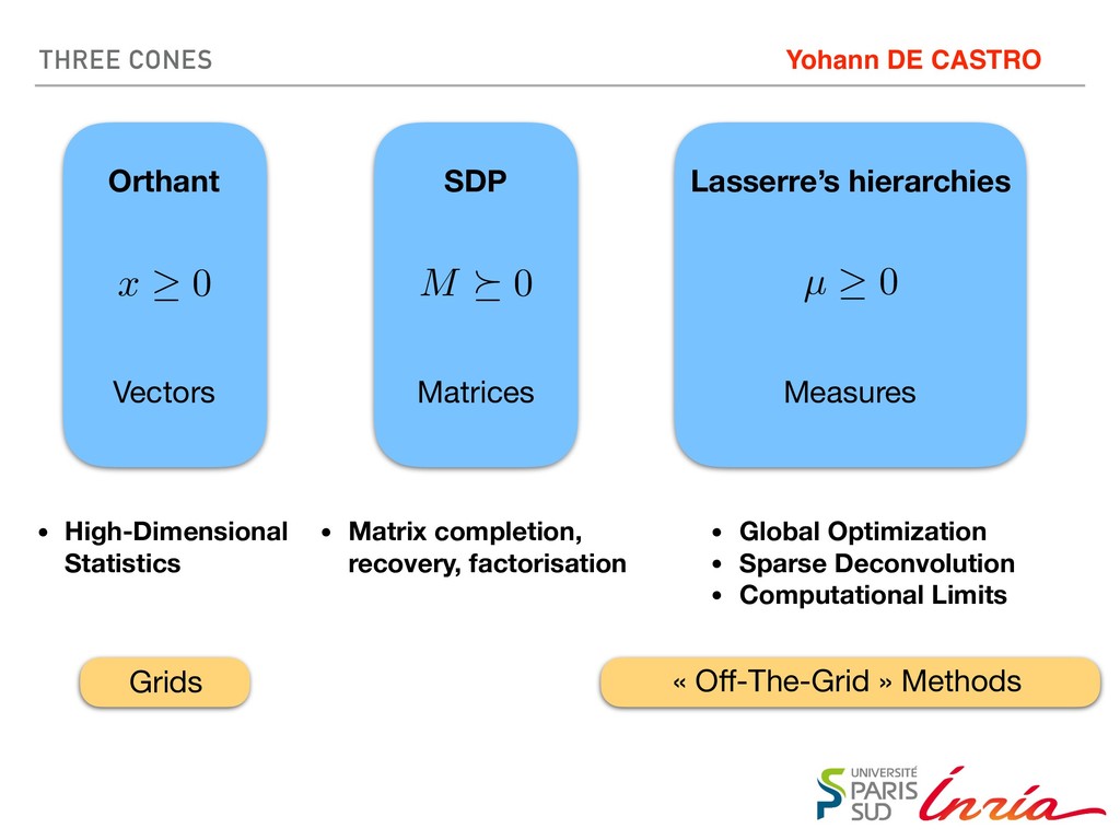
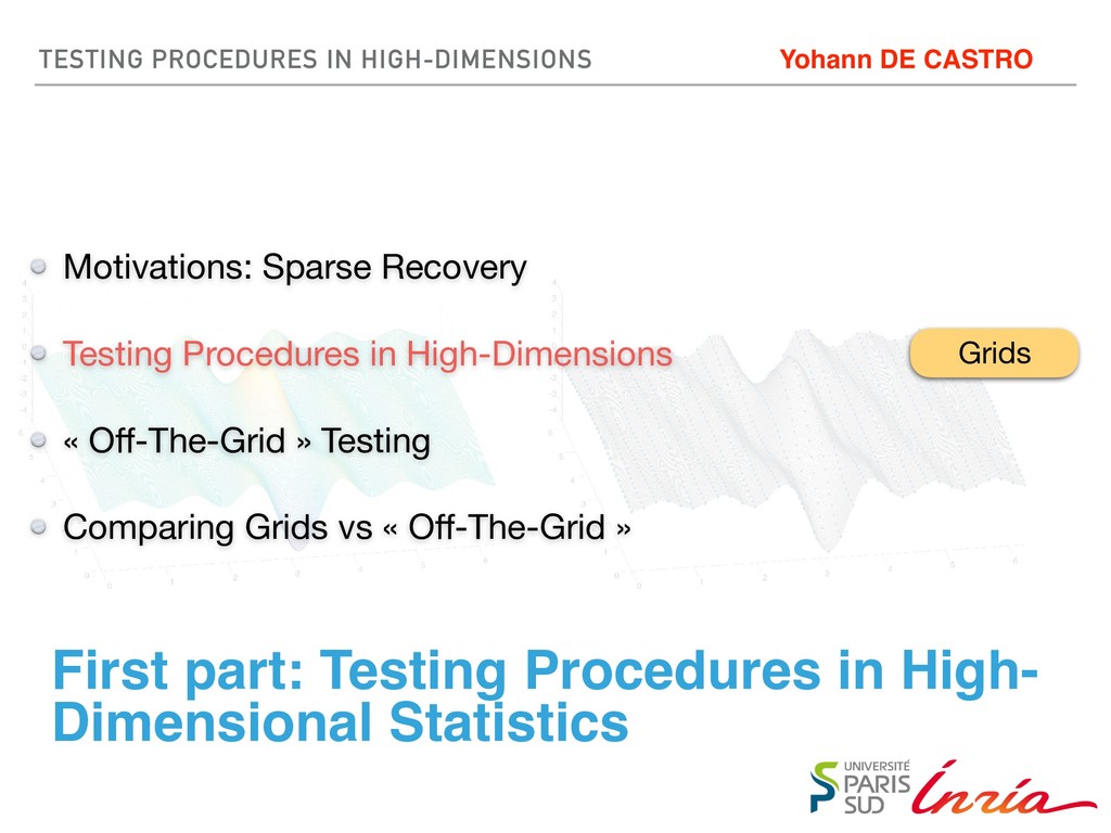
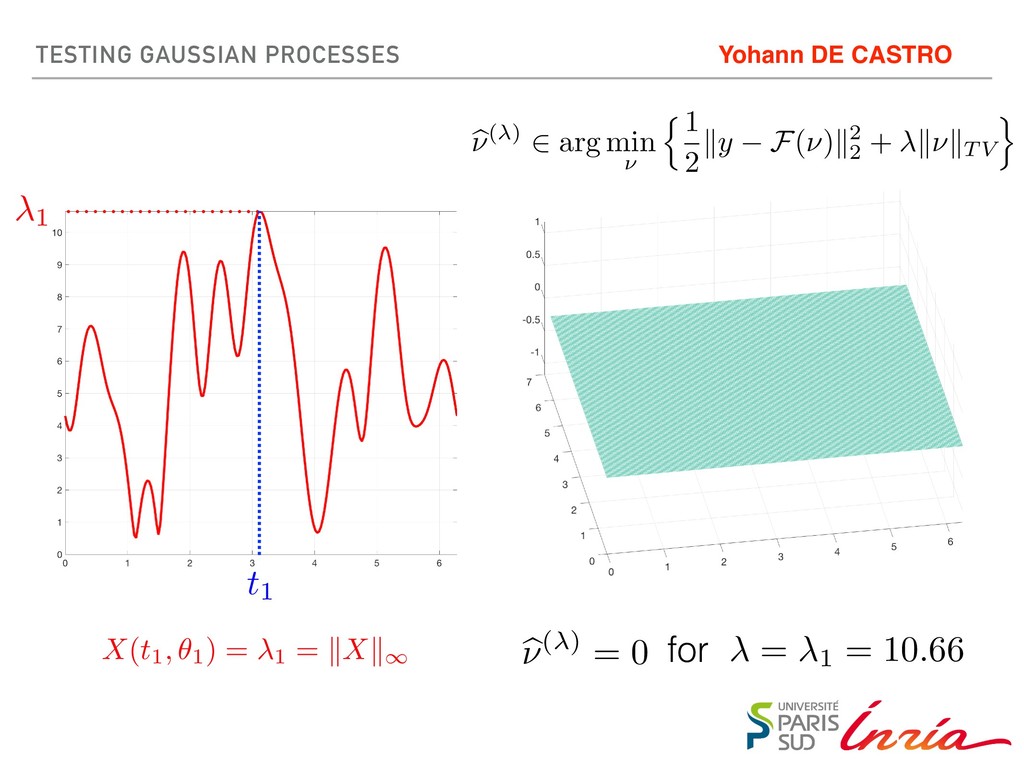
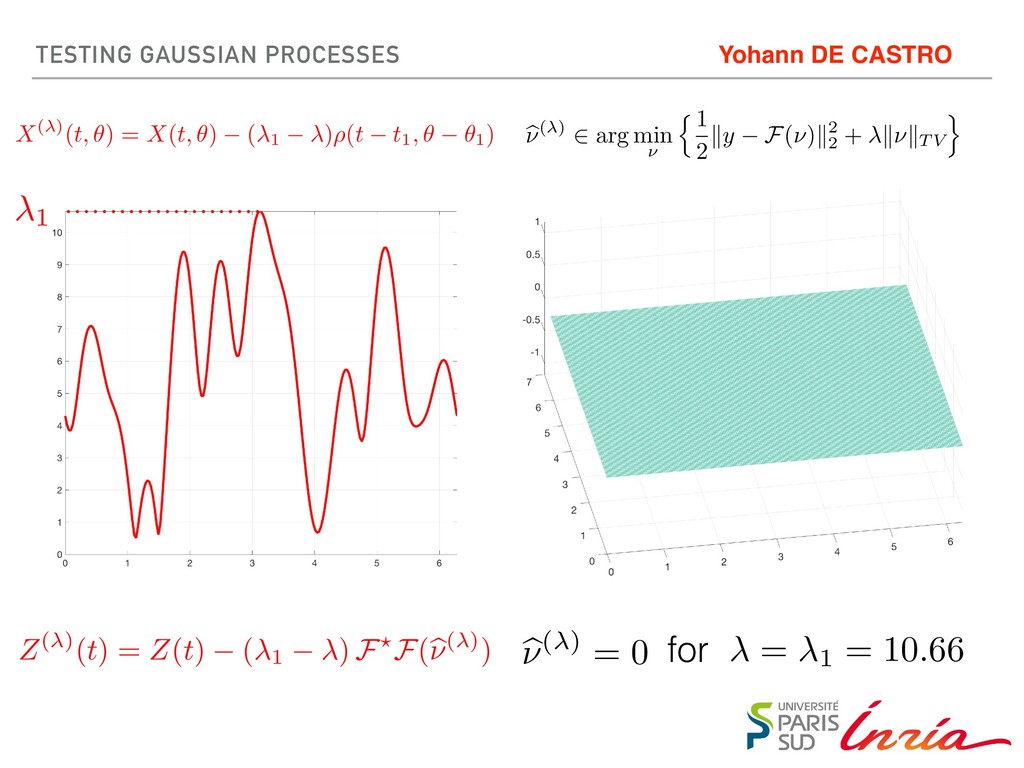
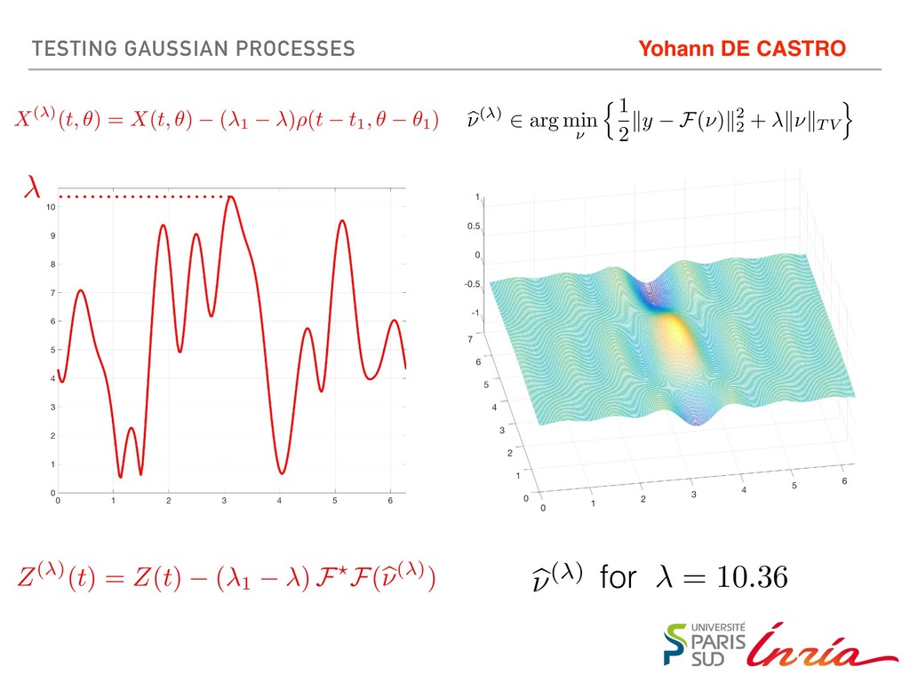
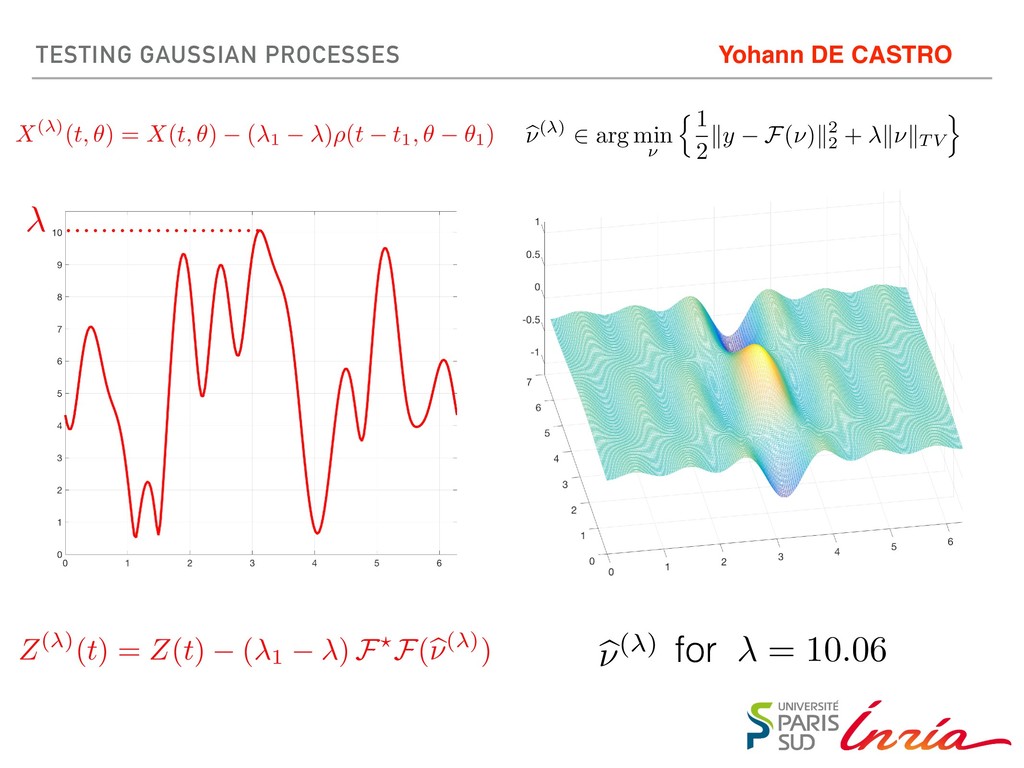
Testing Comparing Grids vs « Off-The-Grid » TESTING PROCEDURES IN HIGH-DIMENSIONS First part: Testing Procedures in High- Dimensional Statistics Yohann DE CASTRO Grids
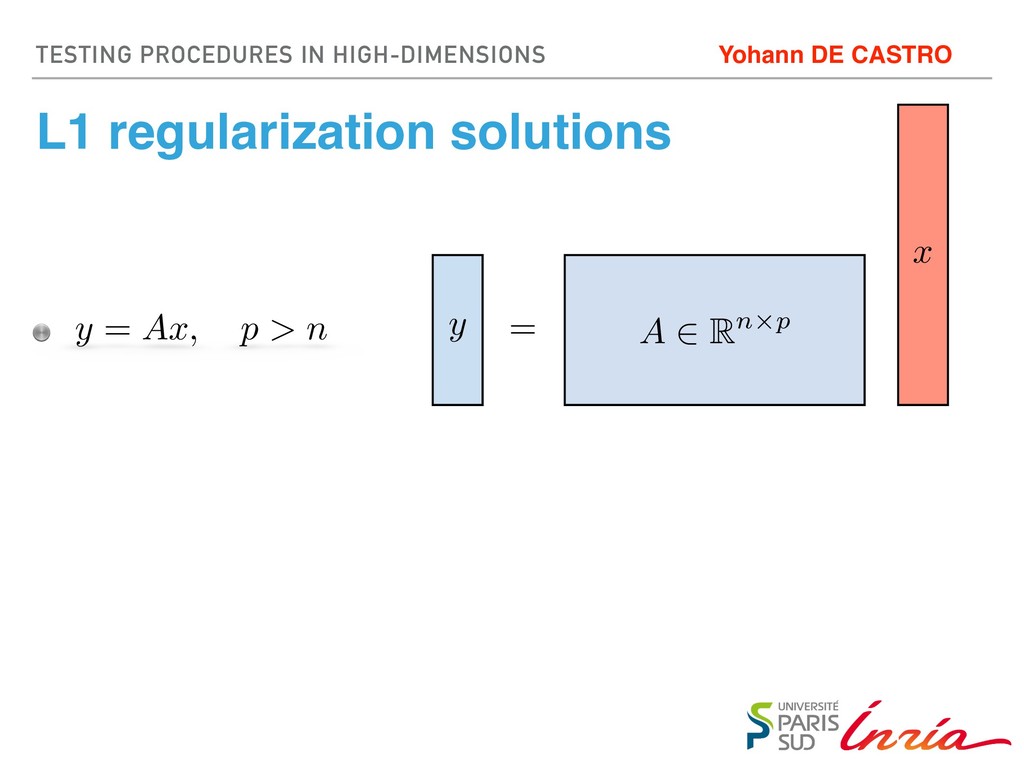
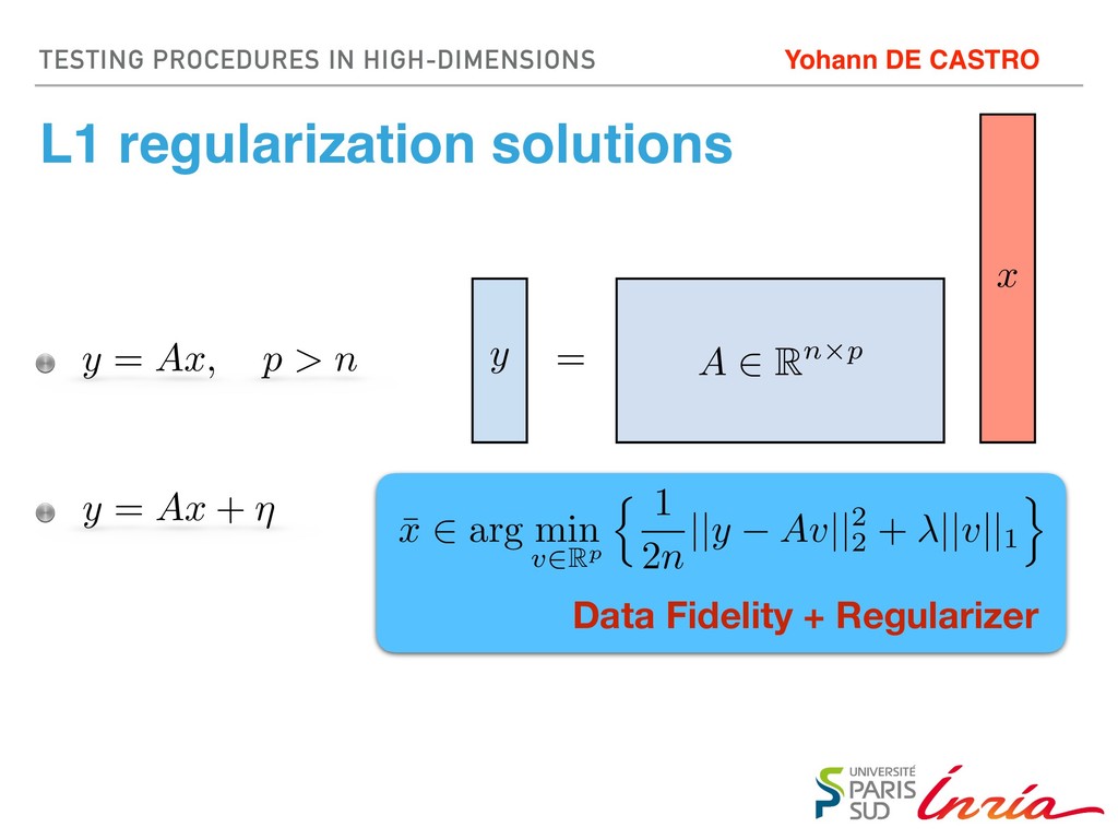
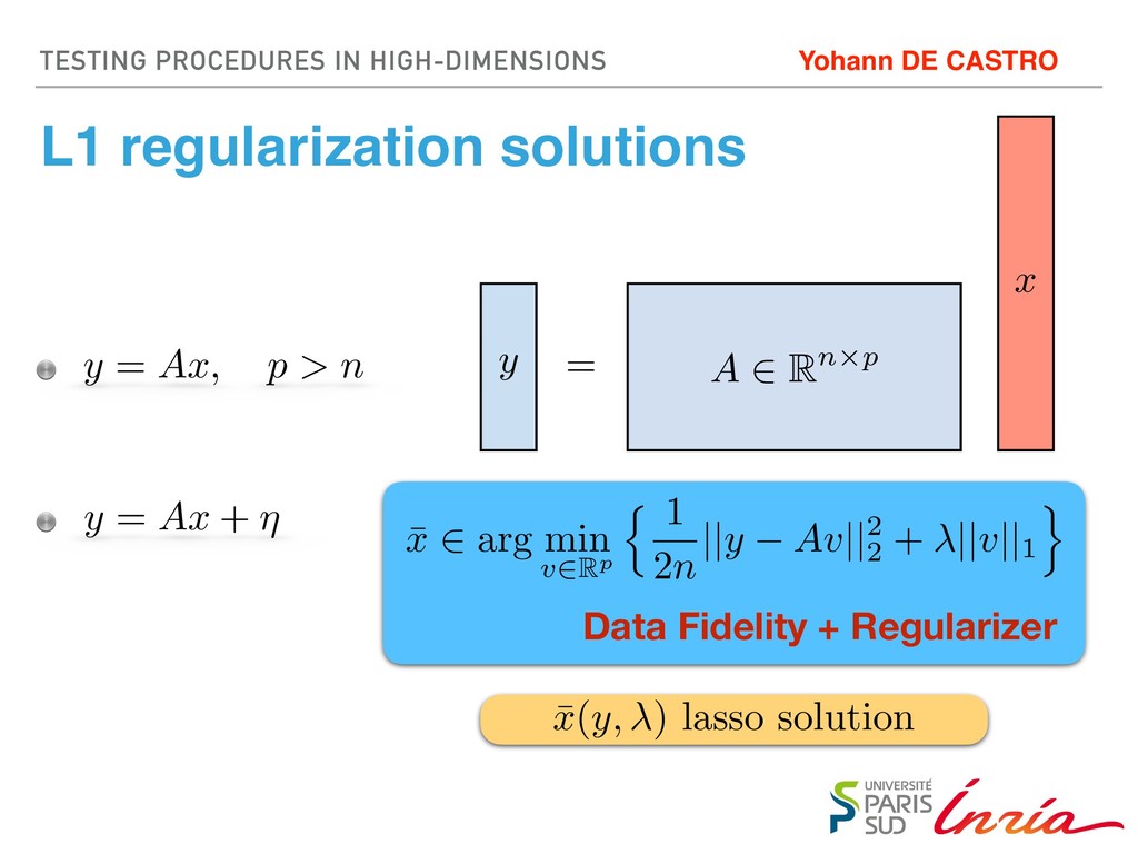
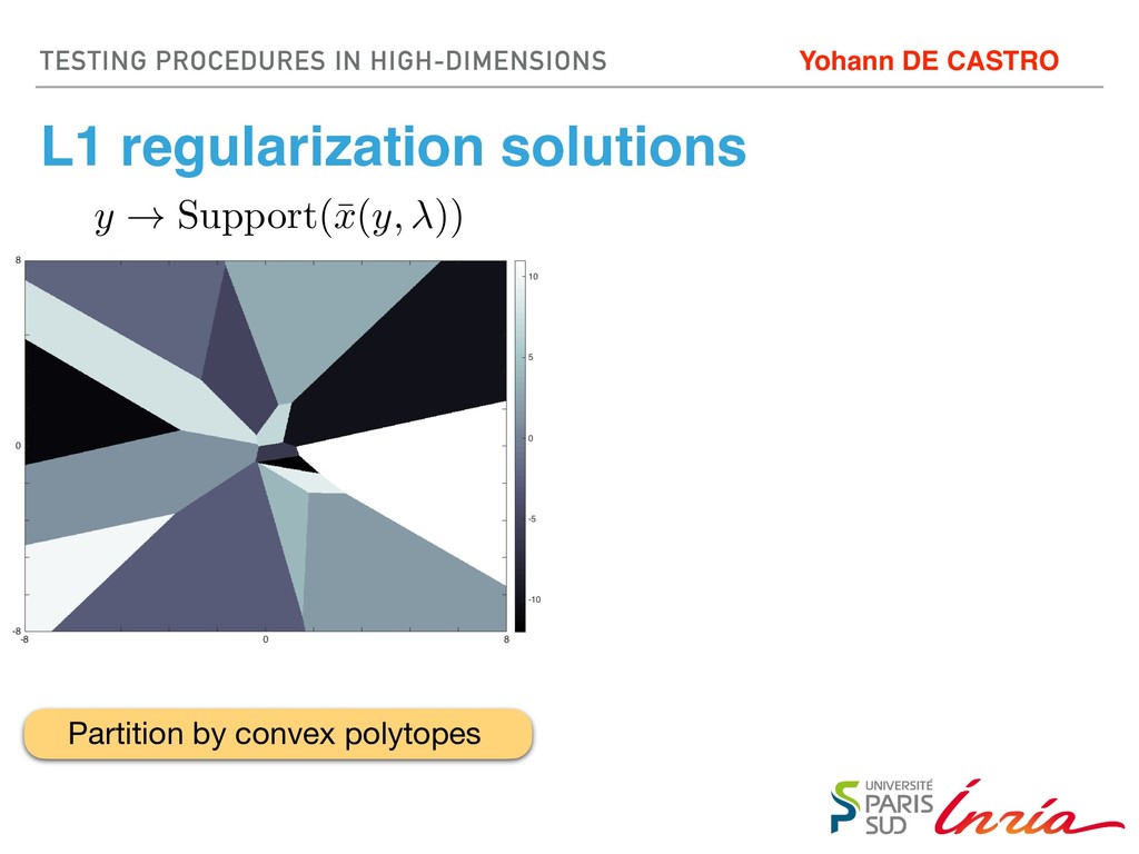
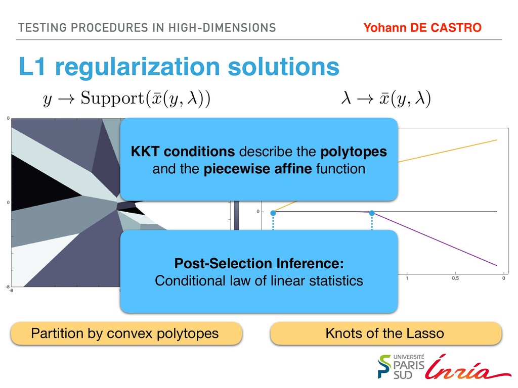
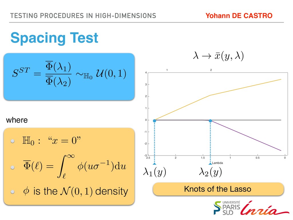
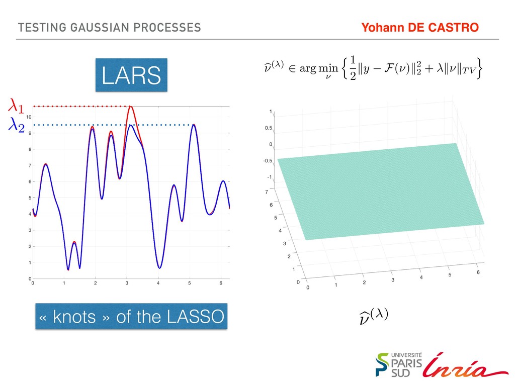
sha1_base64="7CRRBRPjL97NEOm7qp8U4LkTJL8=">AAAC7HicjVHLSsNAFD2N7/qqunQTLGIFKYkIuhTduFS0VmiKTNLRBpNMmEzEUvwEd+7ErT/gVr9D/AP9C++MEXwgOiHJmXPvOTP3Xj+Nwkw5znPJGhgcGh4ZHSuPT0xOTVdmZg8zkcuANwIRCXnks4xHYcIbKlQRP0olZ7Ef8aZ/tq3jzXMus1AkB6qX8nbMTpPwJAyYIuq4stTzlPBiproy7u/naSqkuqx5PpP2Ra234kVk1WHLy8eVqlN3zLJ/ArcAVRRrV1Se4KEDgQA5YnAkUIQjMGT0tODCQUpcG33iJKHQxDkuUSZtTlmcMhixZ/Q9pV2rYBPaa8/MqAM6JaJXktLGImkE5UnC+jTbxHPjrNnfvPvGU9+tR3+/8IqJVegS+5fuI/O/Ol2Lwgk2TA0h1ZQaRlcXFC656Yq+uf2pKkUOKXEadyguCQdG+dFn22gyU7vuLTPxF5OpWb0Pitwcr/qWNGD3+zh/gsPVuuvU3b216uZWMepRzGMBNZrnOjaxg100yPsK93jAo5VY19aNdfueapUKzRy+LOvuDbZGn3E=</latexit> <latexit sha1_base64="7CRRBRPjL97NEOm7qp8U4LkTJL8=">AAAC7HicjVHLSsNAFD2N7/qqunQTLGIFKYkIuhTduFS0VmiKTNLRBpNMmEzEUvwEd+7ErT/gVr9D/AP9C++MEXwgOiHJmXPvOTP3Xj+Nwkw5znPJGhgcGh4ZHSuPT0xOTVdmZg8zkcuANwIRCXnks4xHYcIbKlQRP0olZ7Ef8aZ/tq3jzXMus1AkB6qX8nbMTpPwJAyYIuq4stTzlPBiproy7u/naSqkuqx5PpP2Ra234kVk1WHLy8eVqlN3zLJ/ArcAVRRrV1Se4KEDgQA5YnAkUIQjMGT0tODCQUpcG33iJKHQxDkuUSZtTlmcMhixZ/Q9pV2rYBPaa8/MqAM6JaJXktLGImkE5UnC+jTbxHPjrNnfvPvGU9+tR3+/8IqJVegS+5fuI/O/Ol2Lwgk2TA0h1ZQaRlcXFC656Yq+uf2pKkUOKXEadyguCQdG+dFn22gyU7vuLTPxF5OpWb0Pitwcr/qWNGD3+zh/gsPVuuvU3b216uZWMepRzGMBNZrnOjaxg100yPsK93jAo5VY19aNdfueapUKzRy+LOvuDbZGn3E=</latexit> TESTING PROCEDURES IN HIGH-DIMENSIONS L1 regularization solutions Yohann DE CASTRO ! ¯ x(y, ) <latexit sha1_base64="mekCZGwxlMrNEnNdq+hGpJscFP0=">AAAC4HicjVHLSsNAFD3GV31HXXYTLEIFKYkIuiy6cVnBVsEUmaRTDU2TMJmIpbhw507c+gNu9WvEP9C/8M44gg9EJyQ5c+45Z+bOBFkc5dJ1n0es0bHxicnS1PTM7Nz8gr241MrTQoS8GaZxKo4ClvM4SnhTRjLmR5ngrB/E/DDo7ar64TkXeZQmB3KQ8XafnSZRNwqZJOrELvsxiTvMl6kfMOFcVAfrhlo7sStuzdXD+Qk8Ayowo5HaT/DRQYoQBfrgSCAJx2DI6TmGBxcZcW0MiROEIl3nuMQ0eQtScVIwYnv0PaXZsWETmqvMXLtDWiWmV5DTwSp5UtIJwmo1R9cLnazY37KHOlPtbUD/wGT1iZU4I/Yv34fyvz7Vi0QX27qHiHrKNKO6C01KoU9F7dz51JWkhIw4hTtUF4RD7fw4Z0d7ct27Olum6y9aqVg1D422wKvaJV2w9/06f4LWRs1za97+ZqW+Y666hDJWUKX73EIde2igSdlXuMcDHq3AurZurNt3qTViPMv4Mqy7N6FBmhI=</latexit> <latexit sha1_base64="mekCZGwxlMrNEnNdq+hGpJscFP0=">AAAC4HicjVHLSsNAFD3GV31HXXYTLEIFKYkIuiy6cVnBVsEUmaRTDU2TMJmIpbhw507c+gNu9WvEP9C/8M44gg9EJyQ5c+45Z+bOBFkc5dJ1n0es0bHxicnS1PTM7Nz8gr241MrTQoS8GaZxKo4ClvM4SnhTRjLmR5ngrB/E/DDo7ar64TkXeZQmB3KQ8XafnSZRNwqZJOrELvsxiTvMl6kfMOFcVAfrhlo7sStuzdXD+Qk8Ayowo5HaT/DRQYoQBfrgSCAJx2DI6TmGBxcZcW0MiROEIl3nuMQ0eQtScVIwYnv0PaXZsWETmqvMXLtDWiWmV5DTwSp5UtIJwmo1R9cLnazY37KHOlPtbUD/wGT1iZU4I/Yv34fyvz7Vi0QX27qHiHrKNKO6C01KoU9F7dz51JWkhIw4hTtUF4RD7fw4Z0d7ct27Olum6y9aqVg1D422wKvaJV2w9/06f4LWRs1za97+ZqW+Y666hDJWUKX73EIde2igSdlXuMcDHq3AurZurNt3qTViPMv4Mqy7N6FBmhI=</latexit> <latexit sha1_base64="mekCZGwxlMrNEnNdq+hGpJscFP0=">AAAC4HicjVHLSsNAFD3GV31HXXYTLEIFKYkIuiy6cVnBVsEUmaRTDU2TMJmIpbhw507c+gNu9WvEP9C/8M44gg9EJyQ5c+45Z+bOBFkc5dJ1n0es0bHxicnS1PTM7Nz8gr241MrTQoS8GaZxKo4ClvM4SnhTRjLmR5ngrB/E/DDo7ar64TkXeZQmB3KQ8XafnSZRNwqZJOrELvsxiTvMl6kfMOFcVAfrhlo7sStuzdXD+Qk8Ayowo5HaT/DRQYoQBfrgSCAJx2DI6TmGBxcZcW0MiROEIl3nuMQ0eQtScVIwYnv0PaXZsWETmqvMXLtDWiWmV5DTwSp5UtIJwmo1R9cLnazY37KHOlPtbUD/wGT1iZU4I/Yv34fyvz7Vi0QX27qHiHrKNKO6C01KoU9F7dz51JWkhIw4hTtUF4RD7fw4Z0d7ct27Olum6y9aqVg1D422wKvaJV2w9/06f4LWRs1za97+ZqW+Y666hDJWUKX73EIde2igSdlXuMcDHq3AurZurNt3qTViPMv4Mqy7N6FBmhI=</latexit> <latexit sha1_base64="mekCZGwxlMrNEnNdq+hGpJscFP0=">AAAC4HicjVHLSsNAFD3GV31HXXYTLEIFKYkIuiy6cVnBVsEUmaRTDU2TMJmIpbhw507c+gNu9WvEP9C/8M44gg9EJyQ5c+45Z+bOBFkc5dJ1n0es0bHxicnS1PTM7Nz8gr241MrTQoS8GaZxKo4ClvM4SnhTRjLmR5ngrB/E/DDo7ar64TkXeZQmB3KQ8XafnSZRNwqZJOrELvsxiTvMl6kfMOFcVAfrhlo7sStuzdXD+Qk8Ayowo5HaT/DRQYoQBfrgSCAJx2DI6TmGBxcZcW0MiROEIl3nuMQ0eQtScVIwYnv0PaXZsWETmqvMXLtDWiWmV5DTwSp5UtIJwmo1R9cLnazY37KHOlPtbUD/wGT1iZU4I/Yv34fyvz7Vi0QX27qHiHrKNKO6C01KoU9F7dz51JWkhIw4hTtUF4RD7fw4Z0d7ct27Olum6y9aqVg1D422wKvaJV2w9/06f4LWRs1za97+ZqW+Y666hDJWUKX73EIde2igSdlXuMcDHq3AurZurNt3qTViPMv4Mqy7N6FBmhI=</latexit> 7! A(y, ) 1(y) 2(y) Knots of the Lasso Partition by convex polytopes KKT conditions describe the polytopes and the piecewise affine function Post-Selection Inference: Conditional law of linear statistics
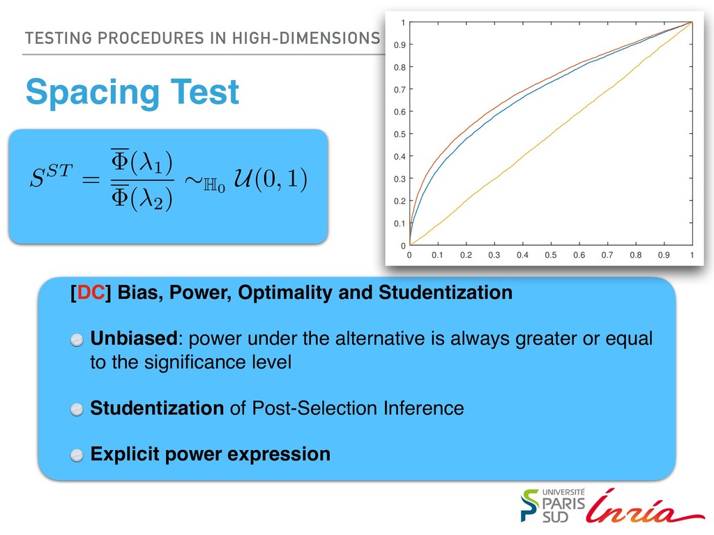
( 2) ⇠ H0 U(0, 1) Yohann DE CASTRO [DC] Bias, Power, Optimality and Studentization Unbiased: power under the alternative is always greater or equal to the significance level Studentization of Post-Selection Inference Explicit power expression 0 0.1 0.2 0.3 0.4 0.5 0.6 0.7 0.8 0.9 1 0 0.1 0.2 0.3 0.4 0.5 0.6 0.7 0.8 0.9 1
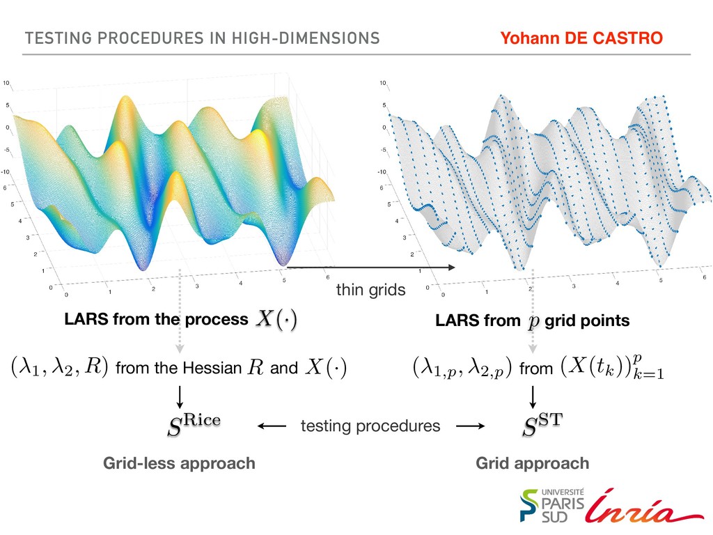
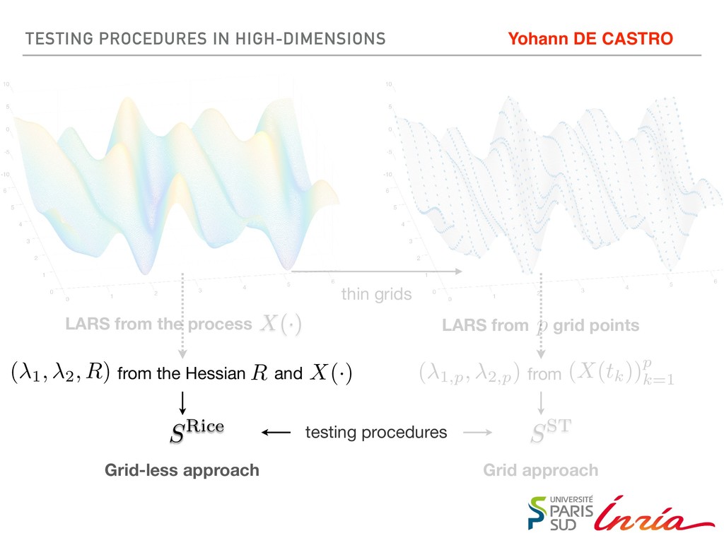
SRice SST from the Hessian and from ( 1, 2, R) R LARS from grid points LARS from the process X(·) testing procedures X(·) (X(tk))p k=1 ( 1,p, 2,p) p Yohann DE CASTRO
SRice SST from the Hessian and from ( 1, 2, R) R LARS from grid points LARS from the process X(·) testing procedures X(·) (X(tk))p k=1 ( 1,p, 2,p) p Yohann DE CASTRO
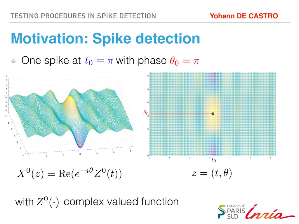
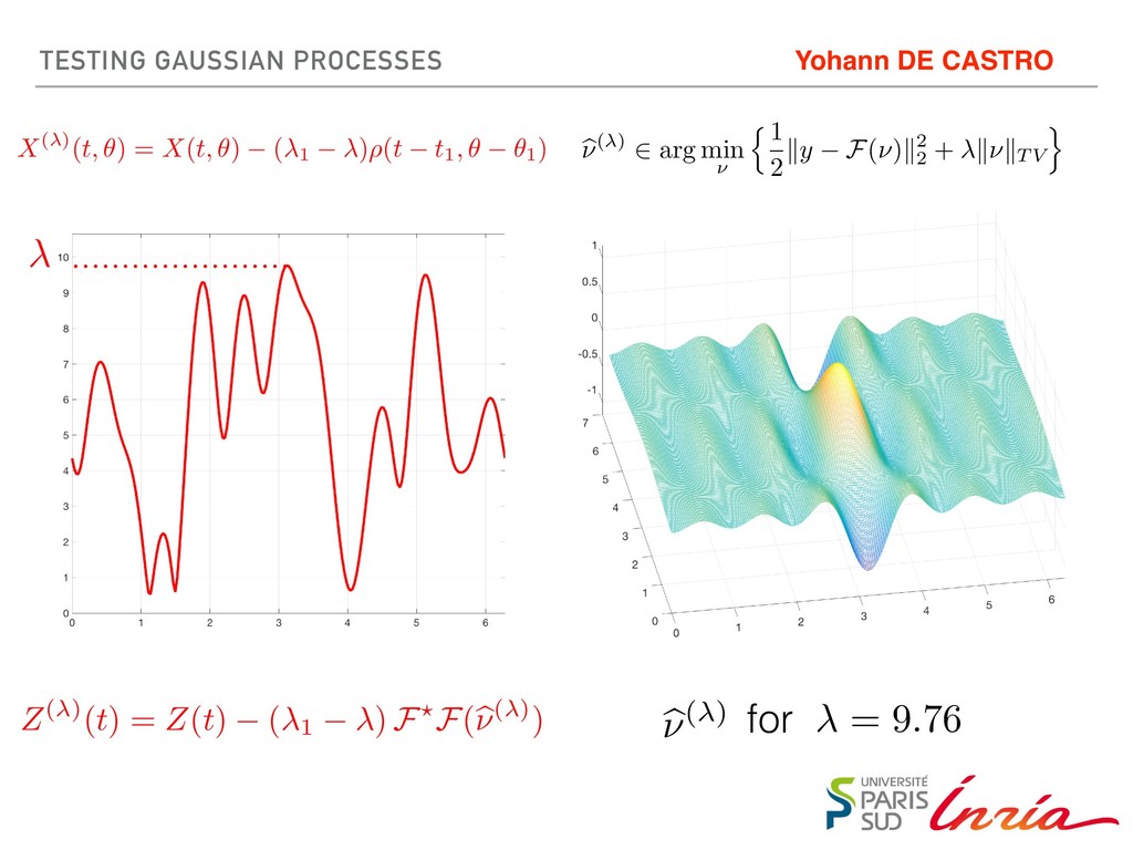
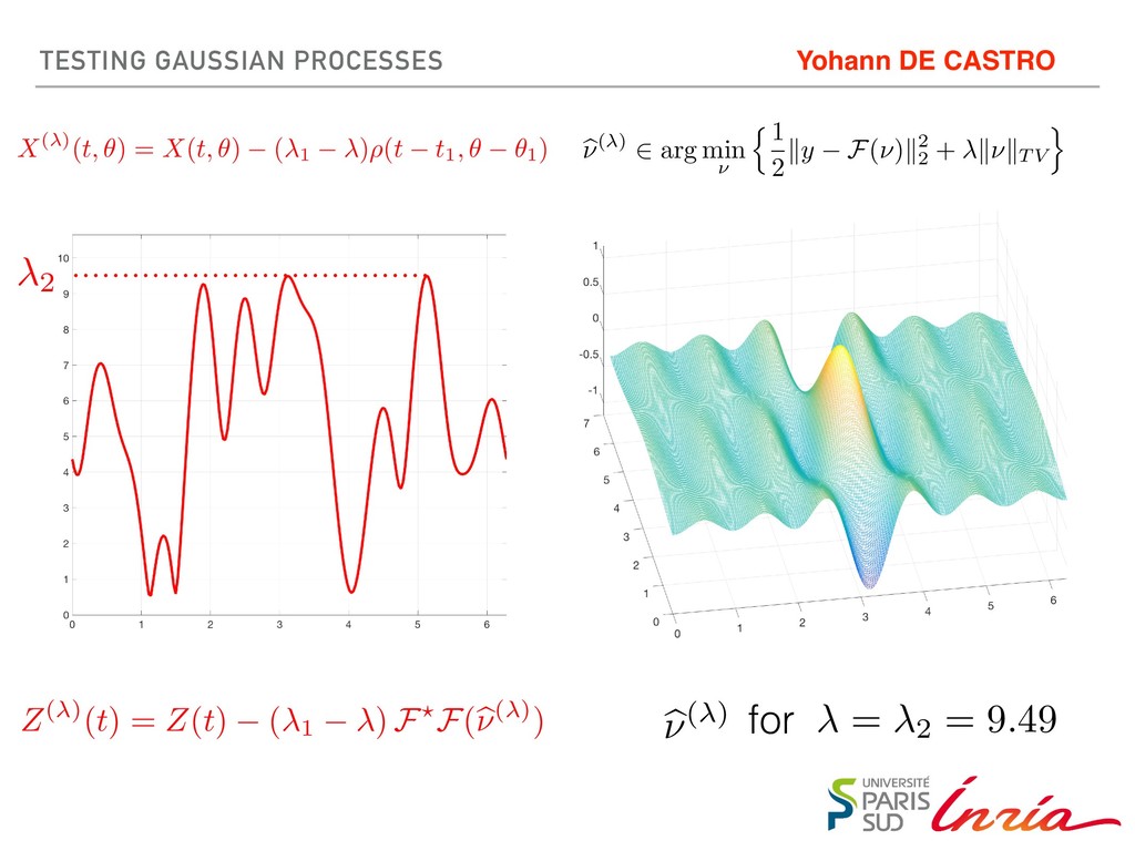
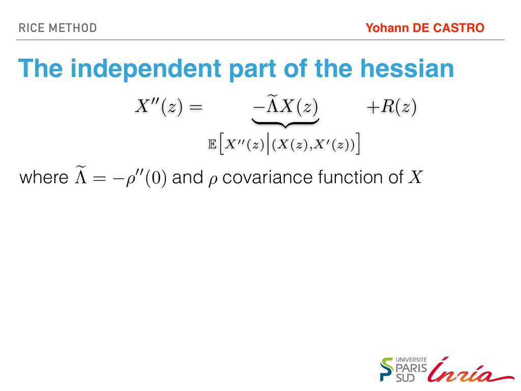
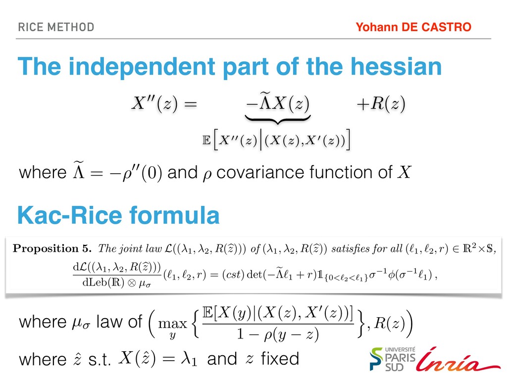
METHOD where Leb(R) denotes the Lebesgue measure on R. As a consequence we can prove the following proposition. Proposition 5. The joint law L(( 1 , 2 , R(b z))) of ( 1 , 2 , R(b z)) satisfies for all (`1 , `2 , r) 2 R2 ⇥S, dL(( 1 , 2 , R(b z))) dLeb(R) ⌦ µ (`1 , `2 , r) = (cst) det( e ⇤`1 + r)1{0<`2<`1} 1 ( 1`1) , where Leb(R) ⌦ µ is defined by (15) and S denotes the set of symmetric matrices. Proof. Observe that the density at point `1 of X(0) with respect to the Lebesgue measure is 1 ( 1`1) and recall (15). Now, for any Borel set B of R2 ⇥ S, note that E h det( e ⇤X(0) + R(0))1{(0< 0 2 <X(0)}1{(X(0), 0 2 ,R(0))2B} i Kac-Rice formula µ where law of The independent part of the hessian ⇣ max y nE[X(y)|(X(z), X0(z))] 1 ⇢(y z) o , R(z) ⌘ e ⇤ = ⇢00(0) where and ⇢ covariance function of X X00(z) = e ⇤X(z) | {z } E ⇥ X00(z) (X(z),X0(z)) ⇤ +R(z) and z fixed ˆ z s.t. X(ˆ z) = 1 where Yohann DE CASTRO
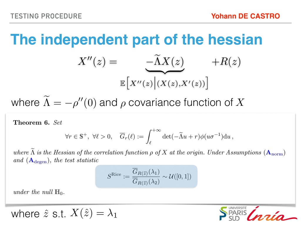
(14), which prove the result. Remark 6. Similarly to the previous computation of the joint distribution of ( 1 , 2 , R(ˆ z)), one can show that under the alternative H1 P(( 1 , 2 , R(z)) 2 B) = (cst) Z T E(| det( e ⇤X(z) + R(z))|10< z 2 <X(z)1(X(z), z 2 ,R(z))2B )dz = (cst) Z B⇥T det( e ⇤l1 + r)10<l2<l1 1(l1 µ(z)) µ ,z(d(l2 , r)) ✓q µ0(z)T e ⇤ 1µ0(z) ◆ dl1dz where µ(·) = E(X(·)) and µ0 denotes the gradient of µ. We can now state our result when the variance is known. Theorem 6. Set 8r 2 S +, 8` > 0, Gr(`) := Z +1 ` det( e ⇤u + r) (u 1)du , where e ⇤ is the Hessian of the correlation function ⇢ of X at the origin. Under Assumptions (Anorm ) and (Adegen ), the test statistic SRice := GR(b z) ( 1) GR(b z) ( 2) ⇠ U([0, 1]) under the null H0 . Proof. Using Proposition 5, we know that the density of 1 at `1 and conditional to ( 2 , R(b z)) = (`2 , r) is equal to The independent part of the hessian e ⇤ = ⇢00(0) where and ⇢ covariance function of X X00(z) = e ⇤X(z) | {z } E ⇥ X00(z) (X(z),X0(z)) ⇤ +R(z) ˆ z s.t. X(ˆ z) = 1 where Yohann DE CASTRO
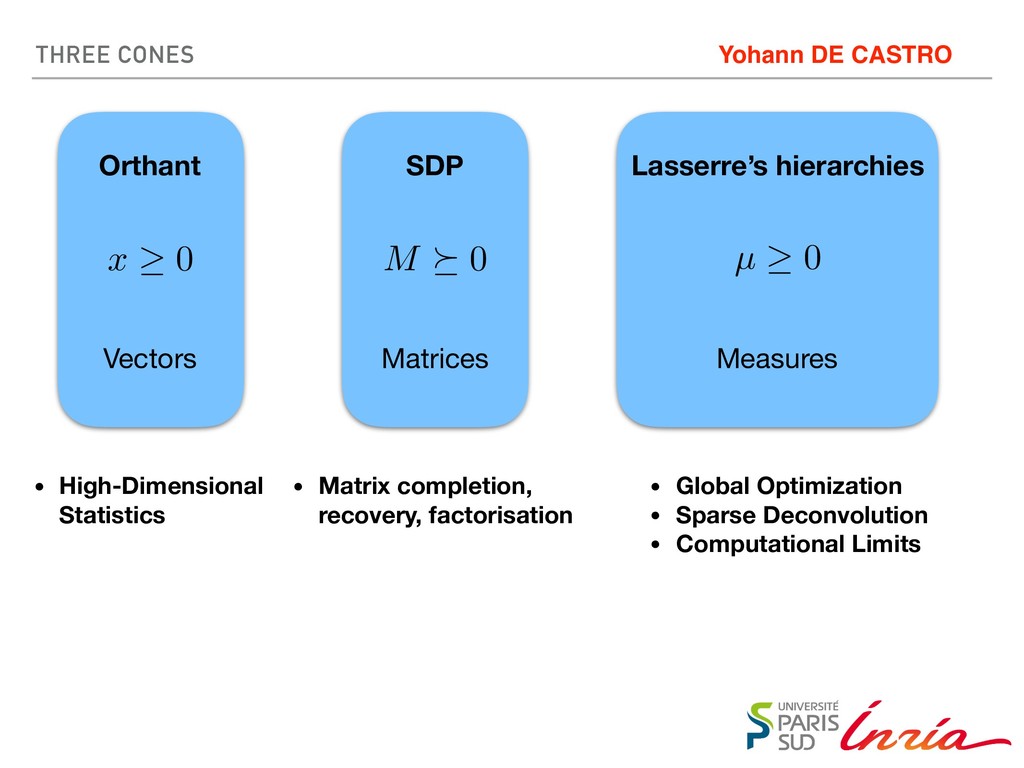
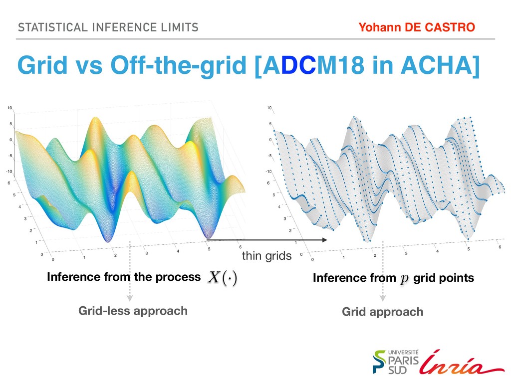
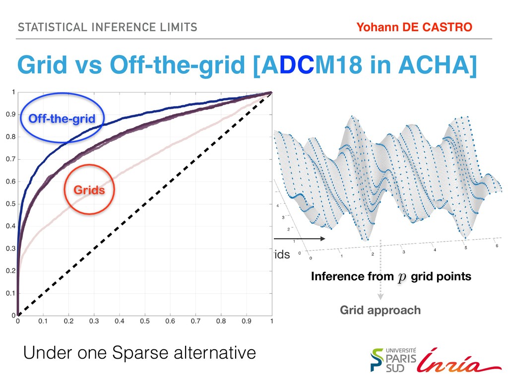
Inference from the process X(·) p Yohann DE CASTRO STATISTICAL INFERENCE LIMITS Grid vs Off-the-grid [ADCM18 in ACHA] Under one Sparse alternative Grids Off-the-grid
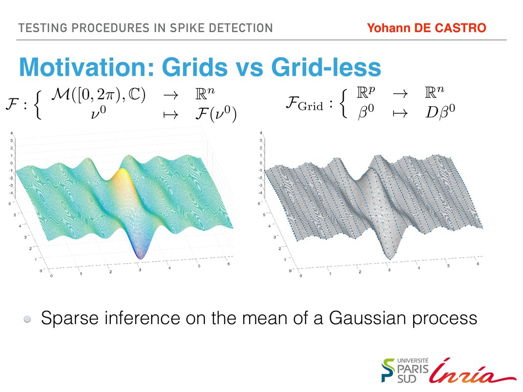
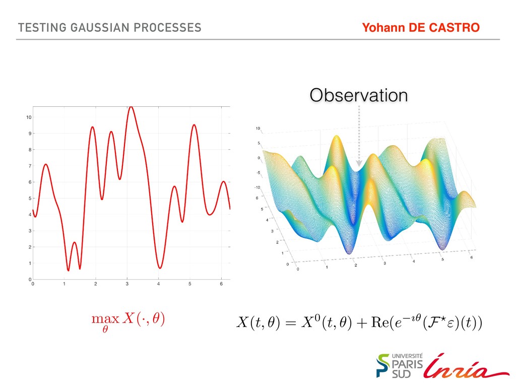
testing procedure on the mean of Gaussian processes Based on L1 MINIMIZATION solutions so that it may detect SPARSE alternatives STUDENTIZATION: no need to know the variance Numerically, the procedure is POWERFUL Computed with SoS HIERARCHIES Studied with Kac-Rice FORMULA Yohann DE CASTRO


 ydecastro
 gpeyre
 eumesy
 murakawatakuya
 youten622
 yumaichikawa
 resolutionfoundation
 institutdelelevage
.png) satai
satai
 hf149
hf149
 lara
lara
 jnunemaker
 sergeychernyshev
 speakerdeck
 portentint
 mkilby
 aleyda
 ryanjones
 szymonslowik
 jct
jct
 raygrieselhuber
 kastner