ImageNet Large Scale Visual Recognition Challenge

Russakovsky, Olga, Jia Deng, Hao Su, Jonathan Krause, Sanjeev Satheesh, Sean Ma, Zhiheng Huang et al. "Imagenet large scale visual recognition challenge." International Journal of Computer Vision 115, no. 3 (2015): 211-252.

Transcript

1. ImageNet Large Scale Visual Recognition Challenge Russakovsky, Olga, et al. International Journal of Computer Vision 115.3 (2015): 211-252 CSci 8980: Special Topics in Vision based Approaches to Learning Presenters: Yeong Hoon Park and Rankyung Hong
2. Outline • Introduction • Challenge tasks • Dataset construction at large scale • Evaluation at large scale • Methods • Results and analysis • Conclusions
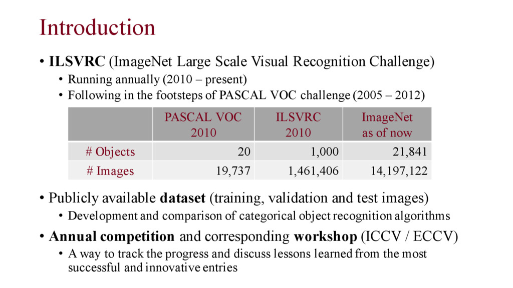
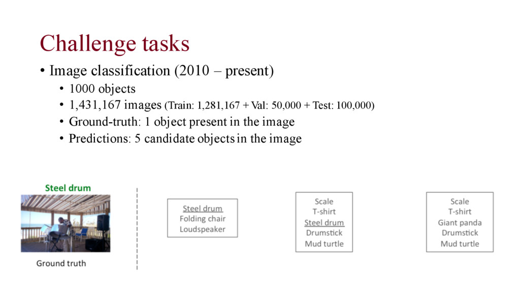
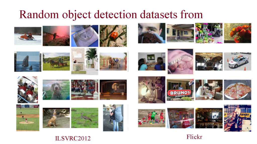
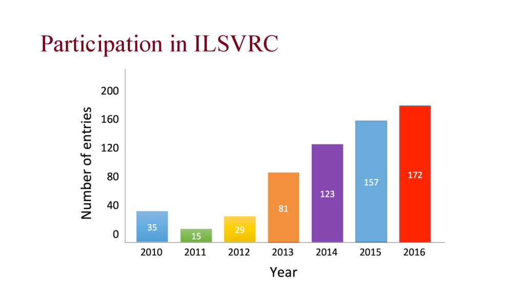
3. Introduction • ILSVRC (ImageNet Large Scale Visual Recognition Challenge) • Running annually (2010 – present) • Following in the footsteps of PASCAL VOC challenge (2005 – 2012) • Publicly available dataset (training, validation and test images) • Development and comparison of categorical object recognition algorithms • Annual competition and corresponding workshop (ICCV / ECCV) • A way to track the progress and discuss lessons learned from the most successful and innovative entries PASCAL VOC 2010 ILSVRC 2010 ImageNet as of now # Objects 20 1,000 21,841 # Images 19,737 1,461,406 14,197,122
4. ILSVRC Challenge tasks • Image classification (2010 – present) • Single-object localization (2011 – present) è Object localization (2014 – present) • Object detection (2013 – present) • Object detection from video (2015 – present) • Scene classification (2015 – present) • Scene parsing (2016 – present)
5. Challenge tasks • Image classification (2010 – present) • 1000 objects • 1,431,167 images (Train: 1,281,167 + Val: 50,000 + Test: 100,000) • Ground-truth: 1 object present in the image • Predictions: 5 candidate objects in the image
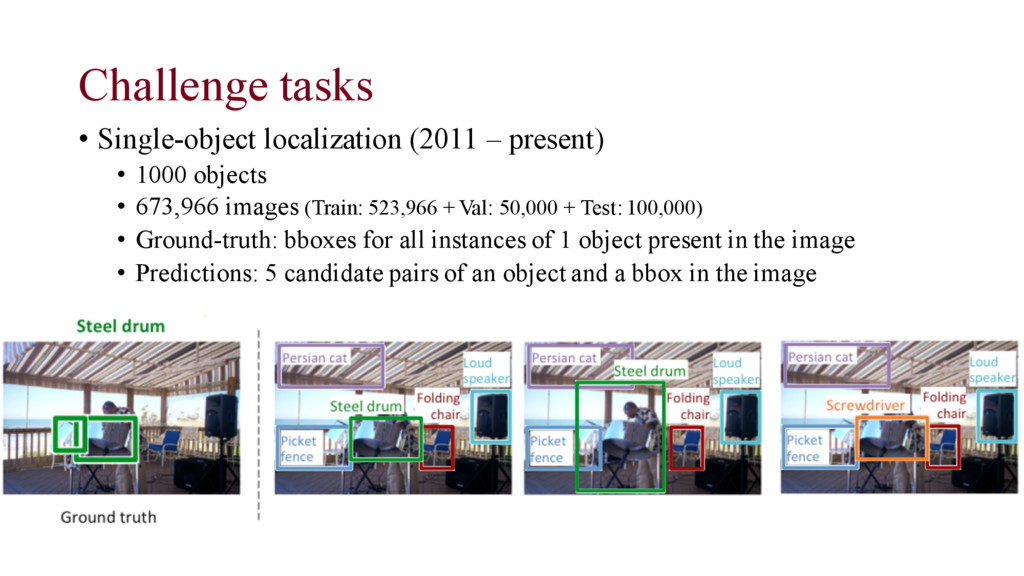
6. Challenge tasks • Single-object localization (2011 – present) • 1000 objects • 673,966 images (Train: 523,966 + Val: 50,000 + Test: 100,000) • Ground-truth: bboxes for all instances of 1 object present in the image • Predictions: 5 candidate pairs of an object and a bbox in the image
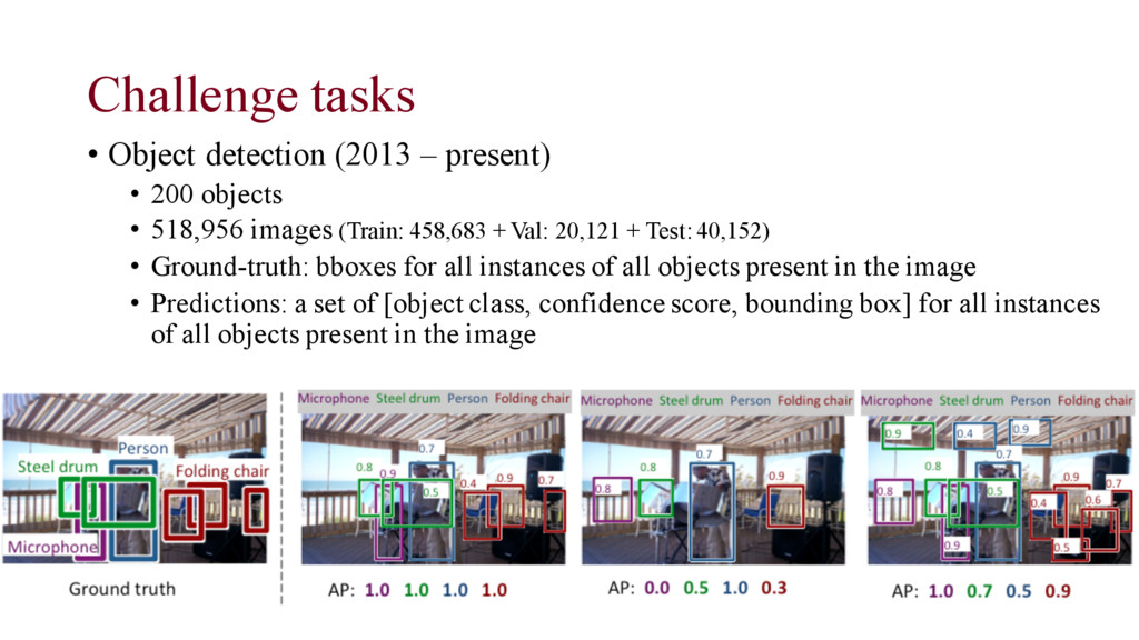
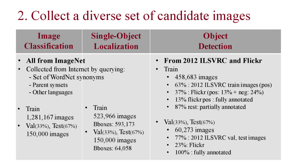
7. Challenge tasks • Object detection (2013 – present) • 200 objects • 518,956 images (Train: 458,683 + Val: 20,121 + Test: 40,152) • Ground-truth: bboxes for all instances of all objects present in the image • Predictions: a set of [object class, confidence score, bounding box] for all instances of all objects present in the image
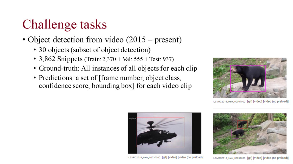
8. Challenge tasks • Object detection from video (2015 – present) • 30 objects (subset of object detection) • 3,862 Snippets (Train: 2,370 + Val: 555 + Test: 937) • Ground-truth: All instances of all objects for each clip • Predictions: a set of [frame number, object class, confidence score, bounding box] for each video clip
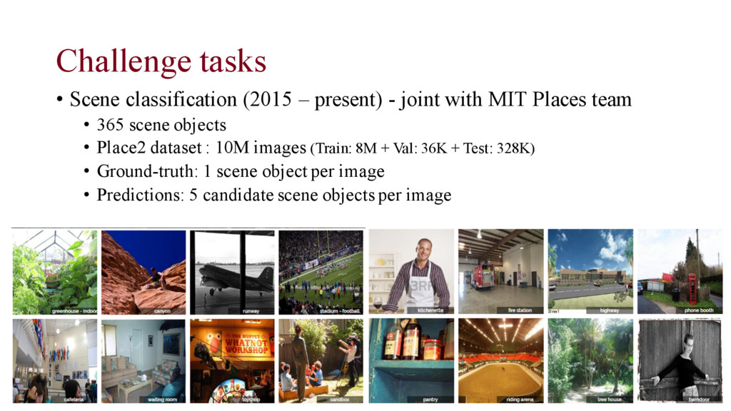
9. Challenge tasks • Scene classification (2015 – present) - joint with MIT Places team • 365 scene objects • Place2 dataset : 10M images (Train: 8M + Val: 36K + Test: 328K) • Ground-truth: 1 scene object per image • Predictions: 5 candidate scene objects per image
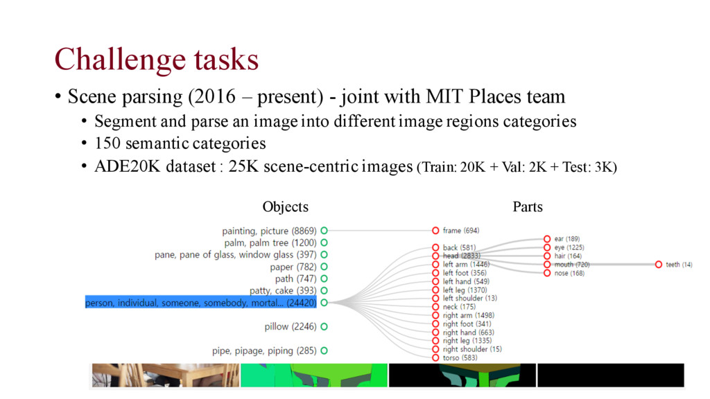
10. Challenge tasks • Scene parsing (2016 – present) - joint with MIT Places team • Segment and parse an image into different image regions categories • 150 semantic categories • ADE20K dataset : 25K scene-centric images (Train: 20K + Val: 2K + Test: 3K) • Ground-truth: All object and part instances are annotated for each image • RGB image (jpg), Object segmentation mask (png) • Part segmentation masks (png) with different levels in hierarchy • Predictions: a semantic segmentation mask, predicting the semantic category for each pixel in the image. Objects Parts
11. Semantic segmentation masks from top 3 participants
12. Dataset construction at large scale 1. Define set of target object categories 2. Collect a diverse set of candidate images 3. Annotate millions of collected images
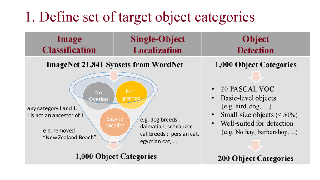
13. 1. Define set of target object categories Image Classification Single-Object Localization Object Detection 1,000 Object Categories Easy to Localize No Overlap Fine- grained ImageNet 21,841 Synsets from WordNet any category I and J, I is not an ancestor of J e.g. removed “New Zealand Beach” e.g. dog breeds : dalmatian, schnauzer, … cat breeds : persian cat, egyptian cat, … • 20 PASCAL VOC • Basic-level objects (e.g. bird, dog, …) • Small size objects (< 50%) • Well-suited for detection (e.g. No hay, barbershop, ...) 1,000 Object Categories 200 Object Categories
14. Many more fine-grained classes
15. 2. Collect a diverse set of candidate images Image Classification Single-Object Localization Object Detection • All from ImageNet • Collected from Internet by querying: - Set of WordNet synonyms - Parent synsets - Other languages • From 2012 ILSVRC and Flickr • Train • 458,683 images • 63% : 2012 ILSVRC train images (pos) • 37% : Flickr (pos: 13% + neg: 24%) • 13% flickr pos : fully annotated • 87% rest: partially annotated • Val(33%), Test(67%) • 60,273 images • 77% : 2012 ILSVRC val, test images • 23%: Flickr • 100% : fully annotated • Train 1,281,167 images • Val(33%), Test(67%) 150,000 images • Train 523,966 images Bboxes: 593,173 • Val(33%), Test(67%) 150,000 images Bboxes: 64,058
16. Diversity of data Low High High Low
17. Random object detection datasets from ILSVRC2012 Flickr
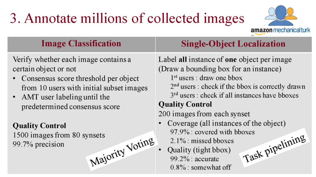
18. 3. Annotate millions of collected images Image Classification Single-Object Localization Verify whether each image contains a certain object or not • Consensus score threshold per object from 10 users with initial subset images • AMT user labeling until the predetermined consensus score Quality Control 1500 images from 80 synsets 99.7% precision Label all instance of one object per image (Draw a bounding box for an instance) 1st users : draw one bbox 2nd users : check if the bbox is correctly drawn 3rd users : check if all instances have bboxes Quality Control 200 images from each synset • Coverage (all instances of the object) 97.9% : covered with bboxes 2.1% : missed bboxes • Quality (tight bbox) 99.2% : accurate 0.8% : somewhat off
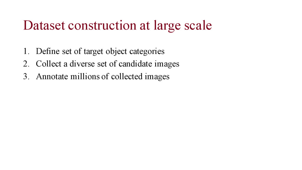
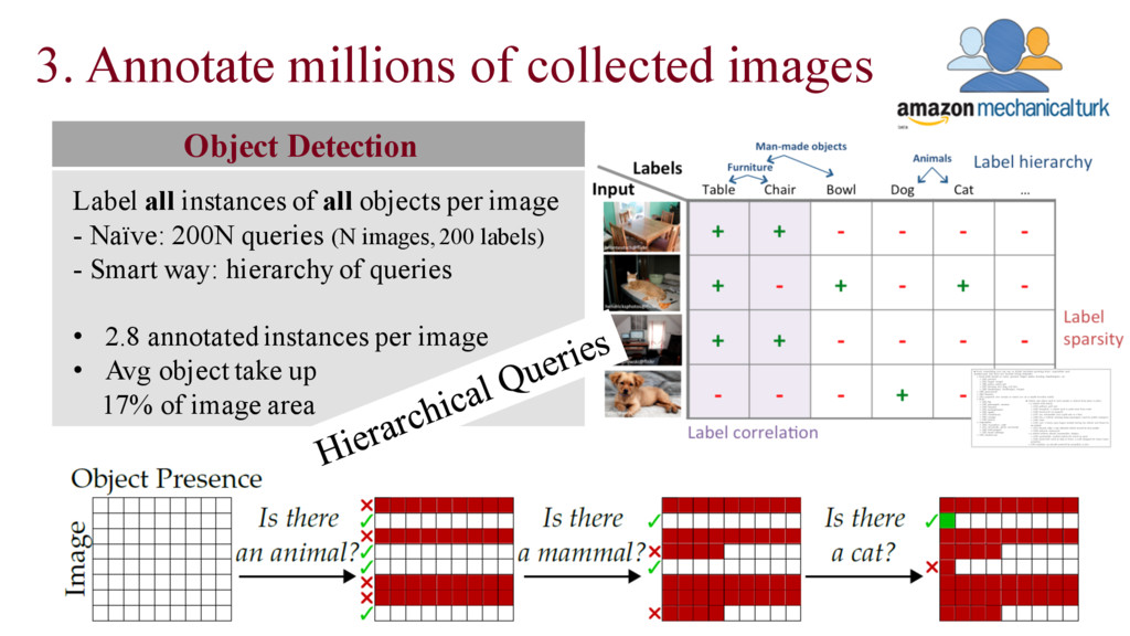
19. Object Detection Label all instances of all objects per image - Naïve: 200N queries (N images, 200 labels) - Smart way: hierarchy of queries • 2.8 annotated instances per image • Avg object take up 17% of image area 3. Annotate millions of collected images
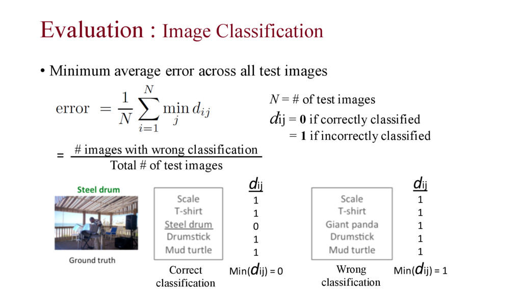
20. • Minimum average error across all test images N = # of test images dij = 0 if correctly classified = 1 if incorrectly classified # images with wrong classification Total # of test images = dij 1 1 0 1 1 Min(dij) = 0 dij 1 1 1 1 1 Min(dij) = 1 Wrong classification Correct classification Evaluation : Image Classification
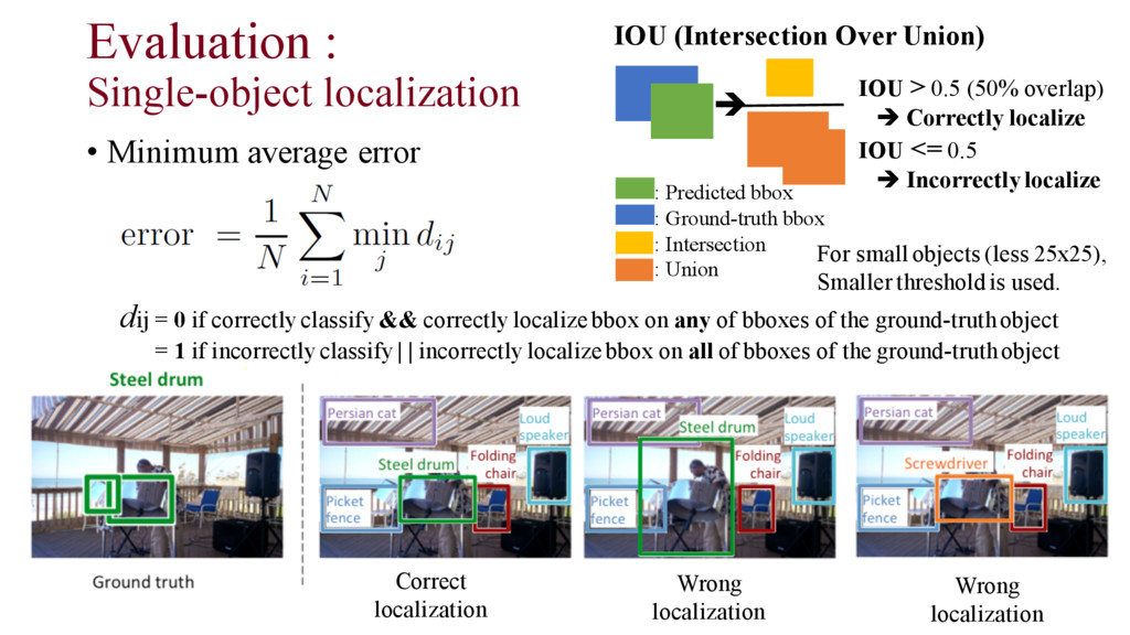
21. Correct localization Wrong localization Wrong localization Evaluation : Single-object localization • Minimum average error dij = 0 if correctly classify && correctly localize bbox on any of bboxes of the ground-truth object = 1 if incorrectly classify | | incorrectly localize bbox on all of bboxes of the ground-truth object : Predicted bbox : Ground-truth bbox : Intersection : Union è IOU > 0.5 (50% overlap) è Correctly localize IOU <= 0.5 è Incorrectly localize IOU (Intersection Over Union) For small objects (less 25x25), Smaller threshold is used.
22. Evaluation : Object Detection • Best accuracy on the most object categories • For each object, the highest average precision(AP) • AP = the area under the precision-recall curve
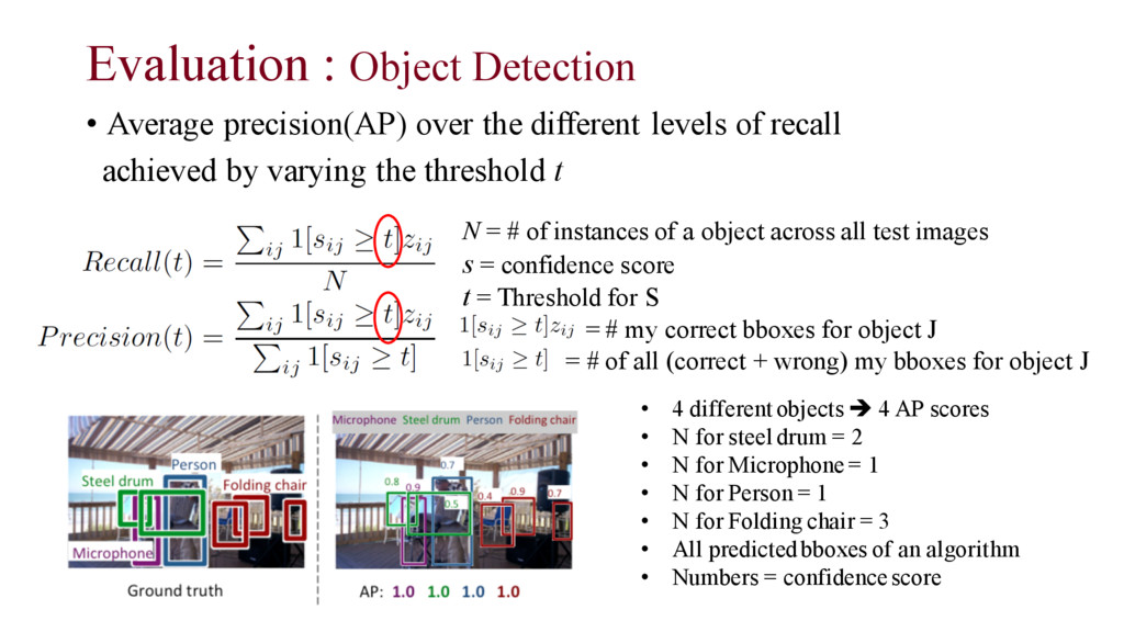
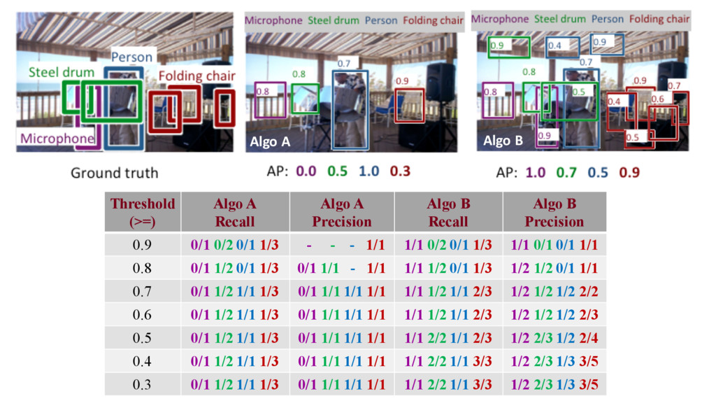
23. Evaluation : Object Detection N = # of instances of a object across all test images s = confidence score t = Threshold for S = # my correct bboxes for object J = # of all (correct + wrong) my bboxes for object J • 4 different objects è 4 AP scores • N for steel drum = 2 • N for Microphone = 1 • N for Person = 1 • N for Folding chair = 3 • All predicted bboxes of an algorithm • Numbers = confidence score • Average precision(AP) over the different levels of recall achieved by varying the threshold t
24. Algo B mAP 0.325 mAP 0.775 Algo A Algo A Algo B
25. Innovation highlights • 2010-2011: SIFT • 2012: AlexNet • 2013: ZFNet, OverFeat • 2014: GoogLeNet, VGGNet • 2015: ResNet
26. SIFT feature extraction Lowe, David G., “Distinctive image features from scale-invariant keypoints,” 2004. Local maxima/minima: candidates for “key point” Scale space
27. SIFT feature extraction
28. ILSVRC 2012 • Deep convolutional neural network
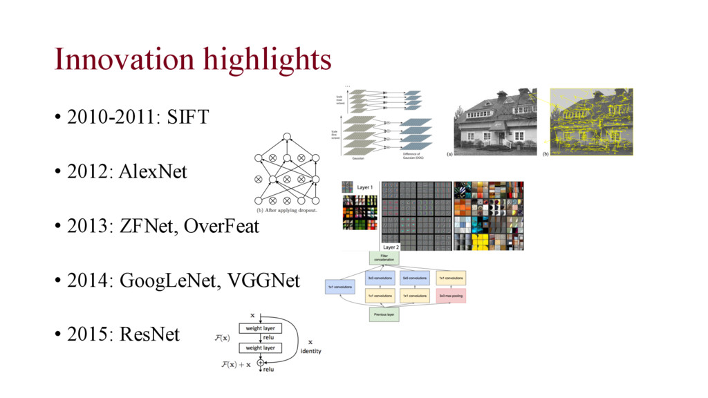
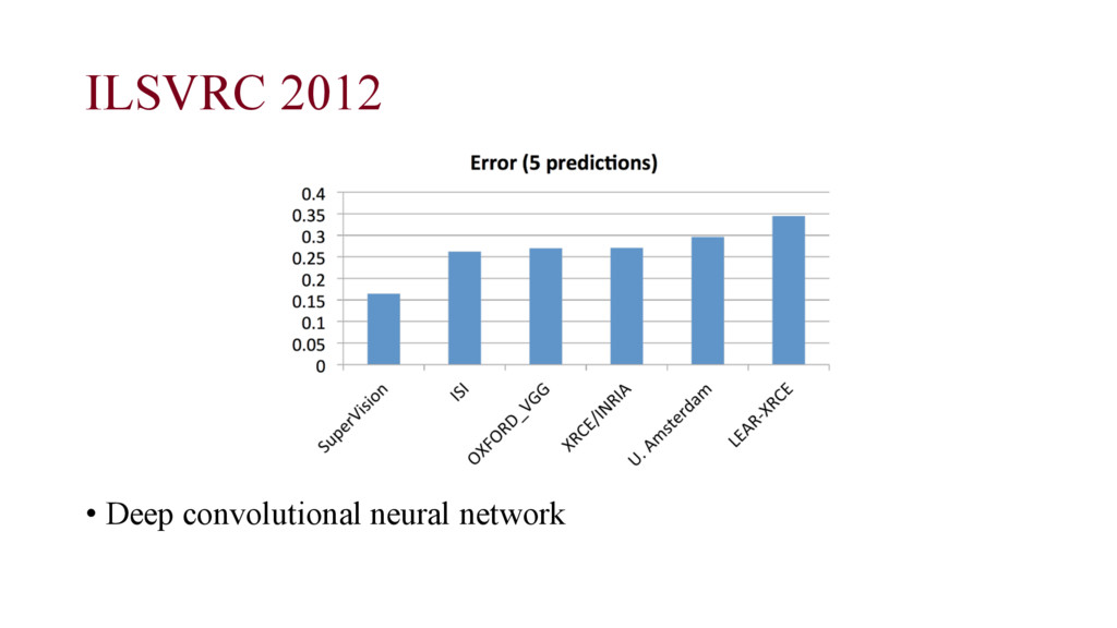
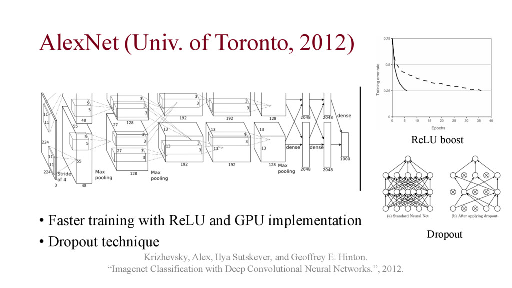
29. AlexNet (Univ. of Toronto, 2012) Krizhevsky, Alex, Ilya Sutskever, and Geoffrey E. Hinton. “Imagenet Classification with Deep Convolutional Neural Networks.”, 2012. • Faster training with ReLU and GPU implementation • Dropout technique ReLU boost Dropout
30. ILSVRC 2013
31. Clarifai/ZFNet (Clarifai/NYU, 2013) Matthew D. Zeiler and Rob Fergus. “Visualizing and Understanding Convolutional Networks”, ECCV 2014. • Visualization of convolution filters
32. Matthew D. Zeiler and Rob Fergus. “Visualizing and Understanding Convolutional Networks”, ECCV 2014.
33. Matthew D. Zeiler and Rob Fergus. “Visualizing and Understanding Convolutional Networks”, ECCV 2014.
34. Matthew D. Zeiler and Rob Fergus. “Visualizing and Understanding Convolutional Networks”, ECCV 2014. Visualizations Help – 2% Boost (a) (b) (c) (d) (e) Needs(renormaliza:on( Too(simple(mid[level( Too(specific(low[level( Dead(filters( Block(Ar:facts( Constrain(RMS( Smaller(Strides( 4(to(2( Smaller(Filters( 7x7(to(11x11(
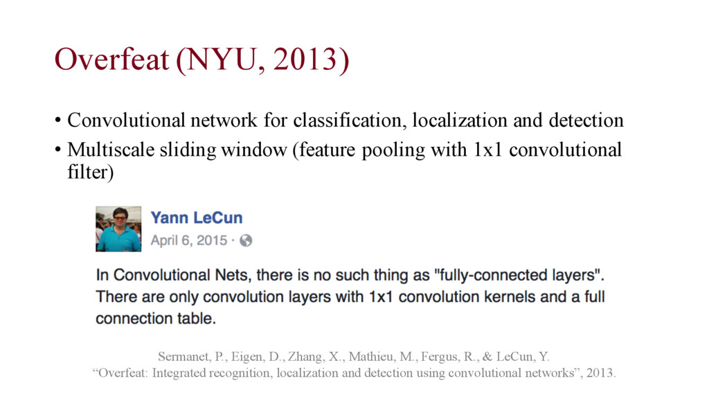
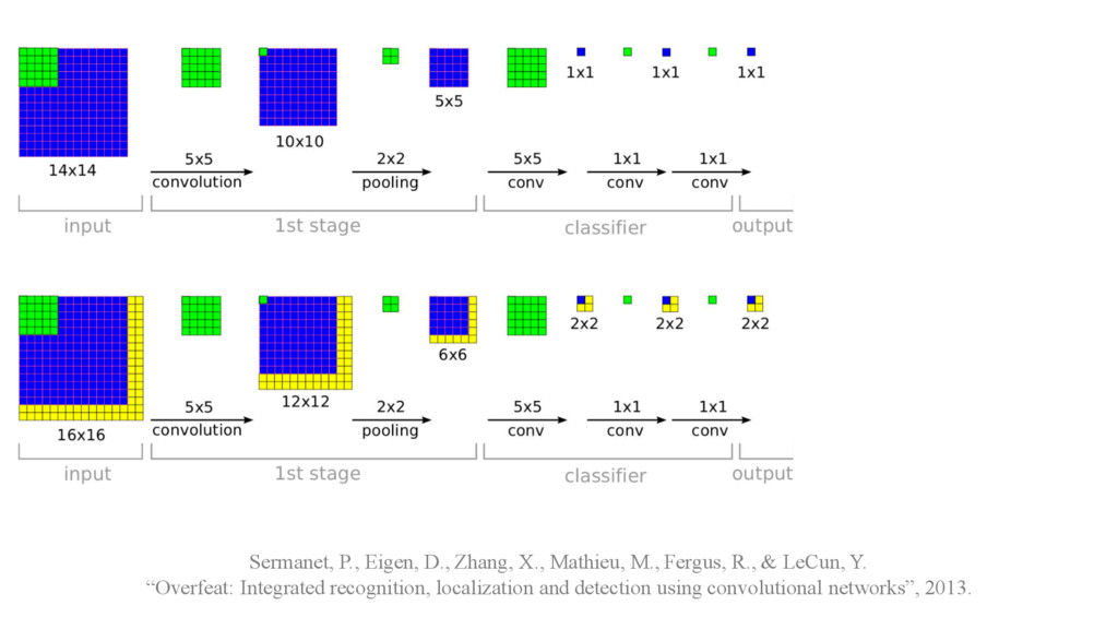
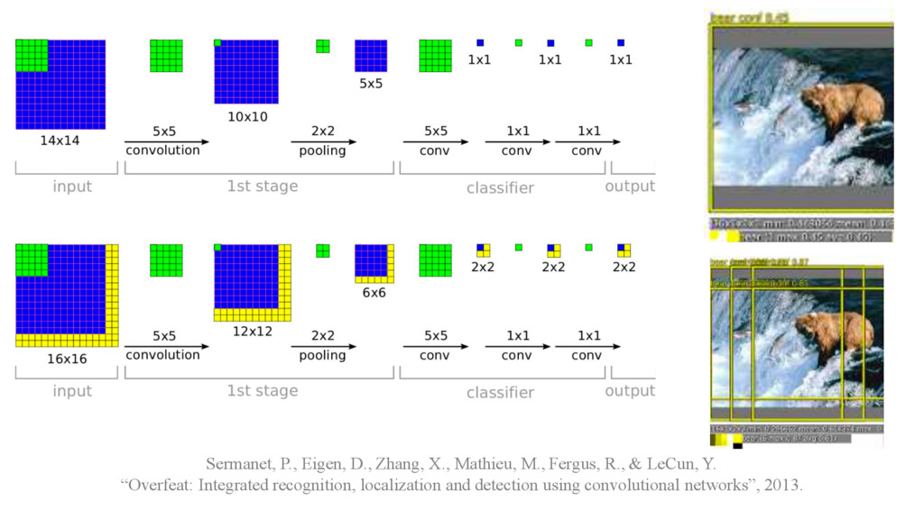
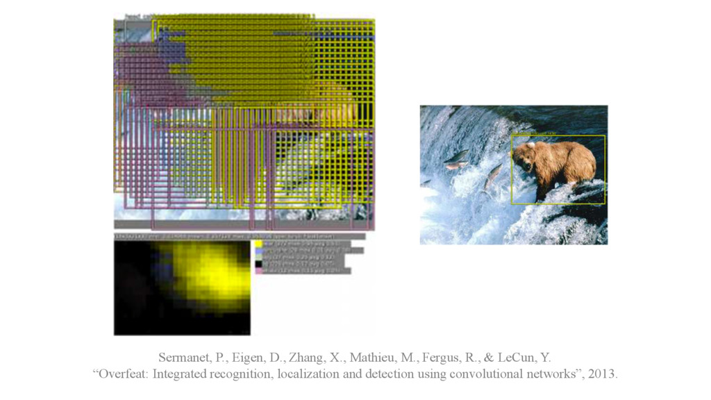
35. Overfeat (NYU, 2013) • Convolutional network for classification, localization and detection • Multiscale sliding window (feature pooling with 1x1 convolutional filter) Sermanet, P., Eigen, D., Zhang, X., Mathieu, M., Fergus, R., & LeCun, Y. “Overfeat: Integrated recognition, localization and detection using convolutional networks”, 2013.
36. Sermanet, P., Eigen, D., Zhang, X., Mathieu, M., Fergus, R., & LeCun, Y. “Overfeat: Integrated recognition, localization and detection using convolutional networks”, 2013.
37. Sermanet, P., Eigen, D., Zhang, X., Mathieu, M., Fergus, R., & LeCun, Y. “Overfeat: Integrated recognition, localization and detection using convolutional networks”, 2013.
38. Sermanet, P., Eigen, D., Zhang, X., Mathieu, M., Fergus, R., & LeCun, Y. “Overfeat: Integrated recognition, localization and detection using convolutional networks”, 2013.
39. GoogLeNet (Google et al, 2014) • 22 layers (compared to 8 layers in ILSVRC 13’) Szegedy, Christian, et al. “Going Deeper with Convolutions ”, CVPR 2015.
40. Inception module • # of features blows up Szegedy, Christian, et al. “Going Deeper with Convolutions ”, CVPR 2015.
41. Inception module Szegedy, Christian, et al. “Going Deeper with Convolutions ”, CVPR 2015. • 1x1 convolutions for dimensionality reduction • Hebbian Principle: “neurons that fire together, wire together”
42. ILSVRC 2015
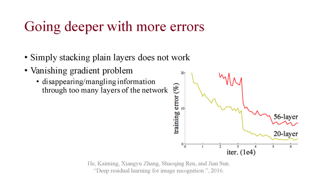
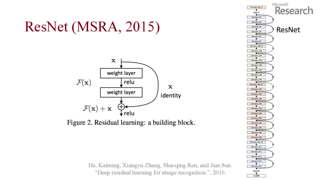
43. Going deeper with more errors • Simply stacking plain layers does not work • Vanishing gradient problem • disappearing/mangling information through too many layers of the network He, Kaiming, Xiangyu Zhang, Shaoqing Ren, and Jian Sun. “Deep residual learning for image recognition.”, 2016.
44. ResNet (MSRA, 2015) He, Kaiming, Xiangyu Zhang, Shaoqing Ren, and Jian Sun. “Deep residual learning for image recognition.”, 2016.
45. Participation in ILSVRC
46. Results
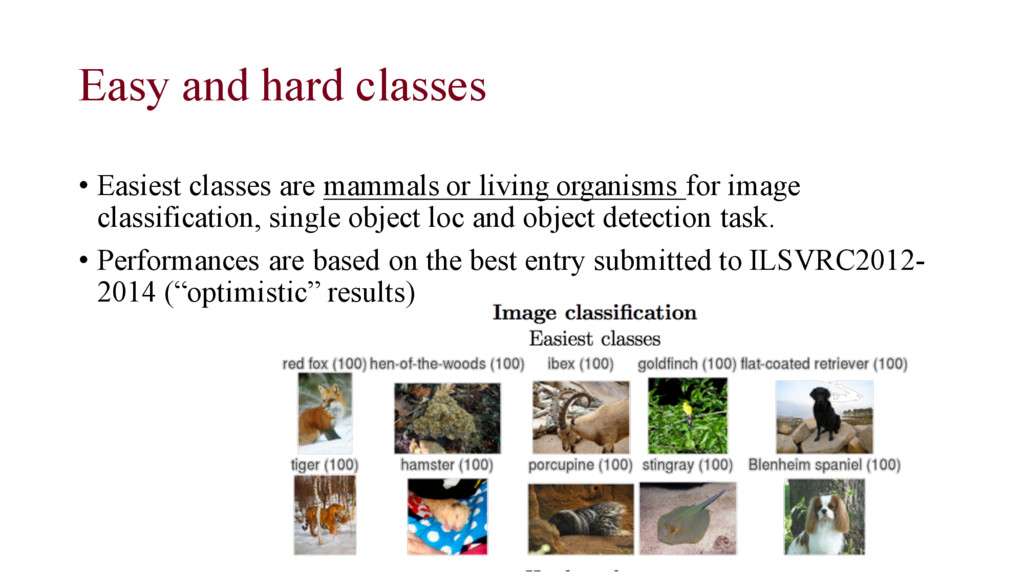
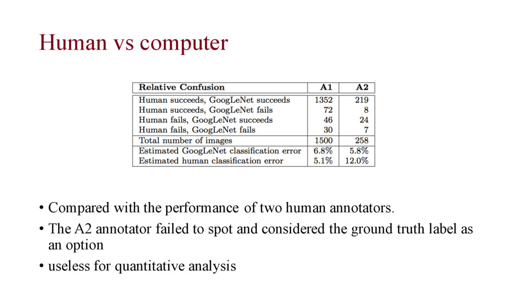
47. Easy and hard classes • Easiest classes are mammals or living organisms for image classification, single object loc and object detection task. • Performances are based on the best entry submitted to ILSVRC2012- 2014 (“optimistic” results)
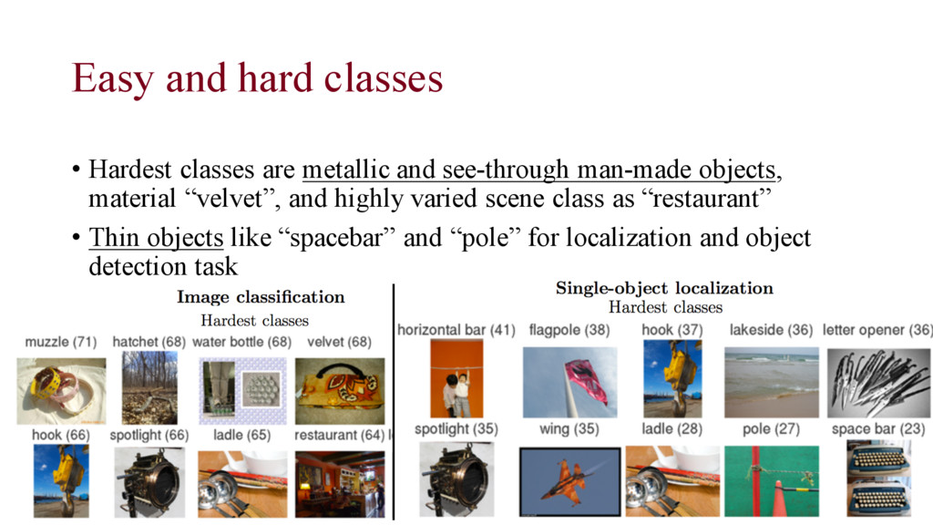
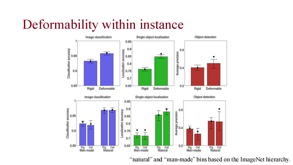
48. Easy and hard classes • Hardest classes are metallic and see-through man-made objects, material “velvet”, and highly varied scene class as “restaurant” • Thin objects like “spacebar” and “pole” for localization and object detection task
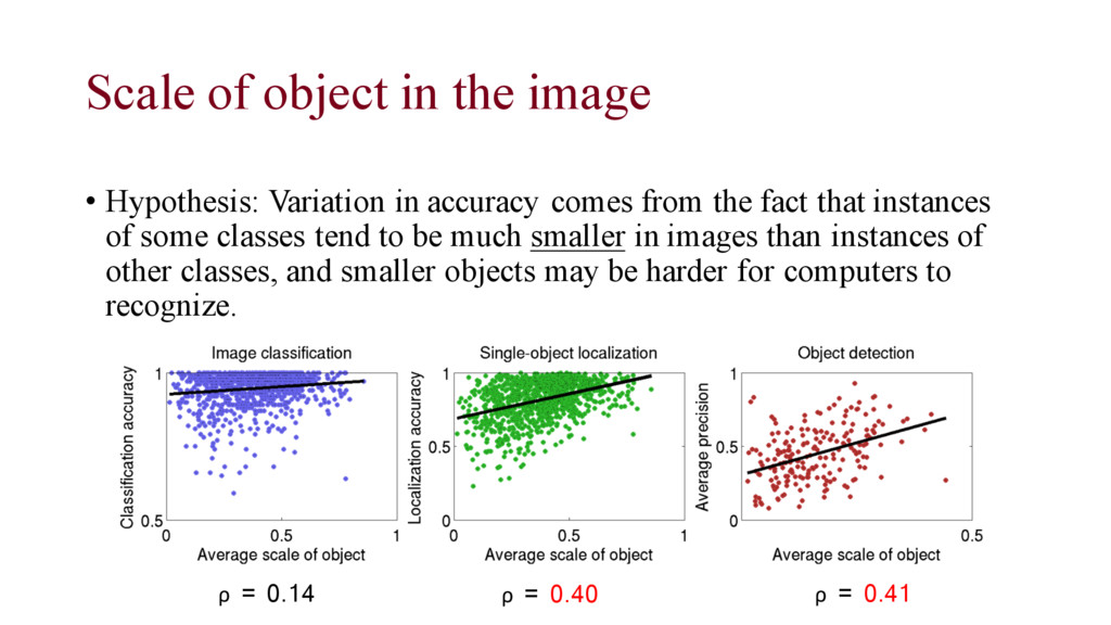
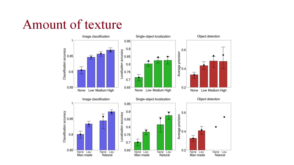
49. Scale of object in the image • Hypothesis: Variation in accuracy comes from the fact that instances of some classes tend to be much smaller in images than instances of other classes, and smaller objects may be harder for computers to recognize. ρ = 0.14 ρ = 0.40 ρ = 0.41
50. Object properties • Real-world object size: XS (nail) to XL (church) • Deformability within instance: rigid (mug) or deformable (water snake) • Amount of texture: none (punching bag) to high (honeycomb)
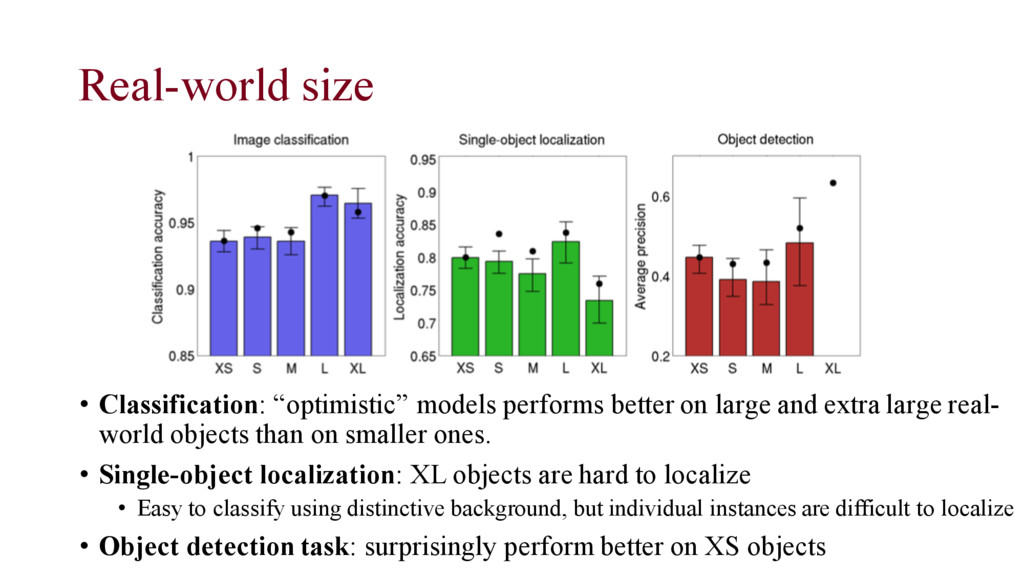
51. Real-world size • Classification: “optimistic” models performs better on large and extra large real- world objects than on smaller ones. • Single-object localization: XL objects are hard to localize • Easy to classify using distinctive background, but individual instances are difficult to localize • Object detection task: surprisingly perform better on XS objects
52. Deformability within instance “natural” and “man-made” bins based on the ImageNet hierarchy.
53. Amount of texture
54. Human vs computer • Compared with the performance of two human annotators. • The A2 annotator failed to spot and considered the ground truth label as an option • useless for quantitative analysis
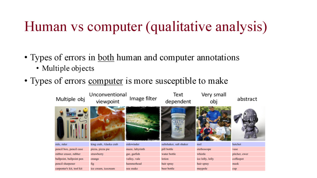
55. Human vs computer (qualitative analysis) • Types of errors in both human and computer annotations • Multiple objects • Types of errors computer is more susceptible to make Multiple obj Unconventional viewpoint Image filter Text dependent Very small obj abstract
56. Human vs computer (qualitative analysis) • Types of errors human is more susceptible to make • Fine-grained recognition (species of dogs) • Class unawareness
57. Conclusions • Lessons of collecting dataset and running the challenges: • All human intelligence tasks need to be exceptionally well-designed. • Crowdsourcing – task design, user interface, etc. • Scaling up the dataset always reveals unexpected challenges.
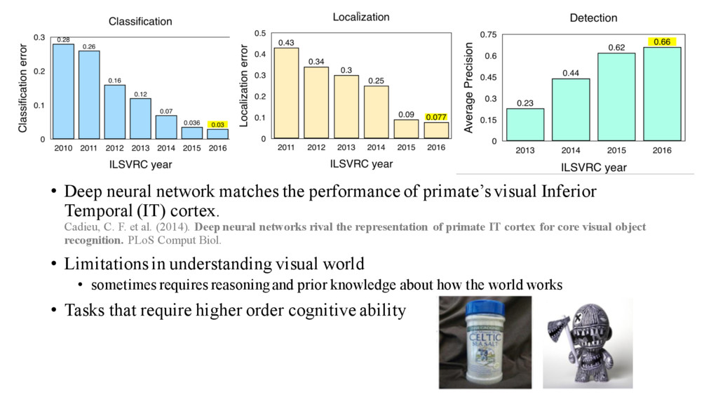
58. • Deep neural network matches the performance of primate’s visual Inferior Temporal (IT) cortex. Cadieu, C. F. et al. (2014). Deep neural networks rival the representation of primate IT cortex for core visual object recognition. PLoS Comput Biol. • Limitations in understanding visual world • sometimes requires reasoning and prior knowledge about how the world works • Tasks that require higher order cognitive ability
59. Questions
61. Threshold (>=) Algo A Recall Algo A Precision Algo B Recall Algo B Precision 0.9 0/1 0/2 0/1 1/3 - - - 1/1 1/1 0/2 0/1 1/3 1/1 0/1 0/1 1/1 0.8 0/1 1/2 0/1 1/3 0/1 1/1 - 1/1 1/1 1/2 0/1 1/3 1/2 1/2 0/1 1/1 0.7 0/1 1/2 1/1 1/3 0/1 1/1 1/1 1/1 1/1 1/2 1/1 2/3 1/2 1/2 1/2 2/2 0.6 0/1 1/2 1/1 1/3 0/1 1/1 1/1 1/1 1/1 1/2 1/1 2/3 1/2 1/2 1/2 2/3 0.5 0/1 1/2 1/1 1/3 0/1 1/1 1/1 1/1 1/1 2/2 1/1 2/3 1/2 2/3 1/2 2/4 0.4 0/1 1/2 1/1 1/3 0/1 1/1 1/1 1/1 1/1 2/2 1/1 3/3 1/2 2/3 1/3 3/5 0.3 0/1 1/2 1/1 1/3 0/1 1/1 1/1 1/1 1/1 2/2 1/1 3/3 1/2 2/3 1/3 3/5 Algo A Algo B