Operating Systems Final Exam Review (ACM2014)

Operating Systems Final Exam Review 陈乐群 2016-12-27

Operating Systems

Windows 2000 Architecture

Processes

– https://en.wikipedia.org/wiki/Process_(computing) “In computing, a process is an instance of
a computer program that is being executed. It contains the program code and its current activity. Depending on the operating system (OS), a process may be made up of multiple threads of execution that execute instructions concurrently.”

Process • Virtualization • CPU • Memory • Set of
Resources • Registers • Address Space • File Descriptors • … • What about execution? • Threads SEC. 2.1 PROCESSES 87 a long enough time interval, all the processes have made progress, but at any giv en instant only one process is actually running. A B C D D C B A Process switch One program counter Four program counters Process Time B C D A (a) (b) (c) Figure 2-1. (a) Multiprogramming four programs. (b) Conceptual model of four independent, sequential processes. (c) Only one program is active at once. In this chapter, we will assume there is only one CPU. Increasingly, howev er, that assumption is not true, since new chips are often multicore, with two, four, or more cores. We will look at multicore chips and multiprocessors in general in Chap. 8, but for the time being, it is simpler just to think of one CPU at a time. So when we say that a CPU can really run only one process at a time, if there are two cores (or CPUs) each of them can run only one process at a time. With the CPU switching back and forth among the processes, the rate at which a process performs its computation will not be uniform and probably not even reproducible if the same processes are run again. Thus, processes must not be pro- grammed with built-in assumptions about timing. Consider, for example, an audio process that plays music to accompany a high-quality video run by another device. Because the audio should start a little later than the video, it signals the video server to start playing, and then runs an idle loop 10,000 times before playing back the audio. All goes well, if the loop is a reliable timer, but if the CPU decides to switch to another process during the idle loop, the audio process may not run again until the corresponding video frames have already come and gone, and the video

Process Creation • System initialization • PID 0 → init
→ everything • Execution of a process-creation system call by a running process • A server daemon accepts a new connection • fork() • A user request to create a new process • Shell / Windowed • Initiation of a batch job

fork() Examples #include <cstdio> #include <unistd.h> #include <sys/types.h> #include <sys/wait.h>
int main() { printf("no flush "); if (fork() == 0) { printf("child\n"); } else { printf("parent\n"); wait(NULL); } } • Output: • no flush parent • no flush child • Because stdio has not ﬂushed yet before fork()

fork() Examples parent: before fork child: before fork grandchild: hi
both child and grandchild: after fork parent, child and grandchild: after fork both child and grandchild: after fork parent, child and grandchild: after fork parent, child and grandchild: after fork #include <cstdio> #include <unistd.h> #include <sys/types.h> #include <sys/wait.h> int main() { pid_t child, grandchild; printf("parent: before fork\n"); if ((child = fork()) == 0) { printf("child: before fork\n"); if ((grandchild = fork()) == 0) { printf("grandchild: hi\n"); } else { waitpid(grandchild, NULL, 0); } printf("both child and grandchild: after fork\n"); } else { waitpid(child, NULL, 0); } printf("parent, child and grandchild: after fork\n"); }

Process Termination • Normal exit (voluntary) • Error exit (voluntary)
• exit() / abort() • Fatal error (involuntary) • x = NULL; y = *x; • Killed by another process (involuntary) • kill() • need permission

Hierarchy • Linux • Process Group • Self: leader •
(Grand-)Children • Session: [Process Groups] • Shares a controlling terminal • Fore-/Back- ground process group • Windows • All processes are created equal • Special token are preserved to control child processes Figure 34-1 shows the process group and session relationships between the vario processes resulting from the execution of the following commands: $ echo $$ Display the PID of the shell 400 $ find / 2> /dev/null | wc -l & Creates 2 processes in background group [1] 659 $ sort < longlist | uniq -c Creates 2 processes in foreground group At this point, the shell (bash), find, wc, sort, and uniq are all running. Figure 34-1: Relationships between process groups, sessions, and the controlling terminal PID = 400 PPID = 399 bash PGID = 400 PPID = 400 find PGID = 658 SID = 400 PID = 659 PPID = 400 wc PGID = 658 SID = 400 PPID = 400 sort PGID = 660 SID = 400 PID = 661 PPID = 400 uniq PGID = 660 SID=400 Process group 660 Session 400 session leader background process groups foreground process group controlling process process group leaders Controlling terminal Foreground PGID = 660 Controlling SID = 400 SID = 400 PID = 660 PID = 658 Process group 658 Process group 400

Process States SEC. 2.1 PROCESSES 93 1 2 3 4
Blocked Running Ready 1. Process blocks for input 2. Scheduler picks another process 3. Scheduler picks this process 4. Input becomes available Figure 2-2. A process can be in running, blocked, or ready state. Transitions between these states are as shown. Four transitions are possible among these three states, as shown. Transition 1 occurs when the operating system discovers that a process cannot continue right now. In some systems the process can execute a system call, such as pause, to get

Process Table SEC. 2.1 PROCESSES 95 Process management Memory management
File management Registers Pointer to text segment info Root directory Program counter Pointer to data segment info Wor king director y Program status word Pointer to stack segment info File descriptors Stack pointer User ID Process state Group ID Pr ior ity Scheduling parameters Process ID Parent process Process group Signals Time when process started CPU time used Children’s CPU time Time of next alarm Figure 2-4. Some of the fields of a typical process-table entry. Context Scheduling Hierarchy

Context Switch 96 PROCESSES AND THREADS CHAP. 2 1. Hardware
stacks program counter, etc. 2. Hardware loads new program counter from interrupt vector. 3. Assembly-language procedure saves registers. 4. Assembly-language procedure sets up new stack. 5. C interrupt service runs (typically reads and buffers input). 6. Scheduler decides which process is to run next. 7. C procedure returns to the assembly code. 8. Assembly-language procedure starts up new current process. Figure 2-5. Skeleton of what the lowest level of the operating system does when an interrupt occurs. A better model is to look at CPU usage from a probabilistic viewpoint. Sup- pose that a process spends a fraction p of its time waiting for I/O to complete. With

System Calls 52 INTRODUCTION CHAP. 1 Return to caller 4
10 6 0 9 7 8 3 2 1 11 Dispatch Sys call handler Address 0xFFFFFFFF User space Kernel space (Operating system) Library procedure read User program calling read Trap to the kernel Put code for read in register Increment SP Call read Push fd Push &buffer Push nbytes 5 Figure 1-17. The 11 steps in making the system call read(fd, buffer, nbytes).

Degree of Multiprogramming • I/O-bound • Larger degree • Better
util • CPU-bound • Larger degree • Heavier scheduler • May be slower 4. Assembly-language procedure sets up new stack. 5. C interrupt service runs (typically reads and buffers input). 6. Scheduler decides which process is to run next. 7. C procedure returns to the assembly code. 8. Assembly-language procedure starts up new current process. Figure 2-5. Skeleton of what the lowest level of the operating system does when an interrupt occurs. A better model is to look at CPU usage from a probabilistic viewpoint. Sup- pose that a process spends a fraction p of its time waiting for I/O to complete. With n processes in memory at once, the probability that all n processes are waiting for I/O (in which case the CPU will be idle) is pn. The CPU utilization is then given by the formula CPU utilization = 1 − pn Figure 2-6 shows the CPU utilization as a function of n, which is called the degree of multiprogramming. 50% I/O wait 80% I/O wait 20% I/O wait 100 80 60 40 20 1 2 3 4 5 6 7 8 9 10 0 Degree of multiprogramming CPU utilization (in percent) Figure 2-6. CPU utilization as a function of the number of processes in memory.

Threads

Threads • An understanding • Lightweight Process • Shared address
space • But I prefer …

Threads • Processes • Virtualization • CPU • Memory •
Set of Resources • Registers • Address Space • File Descriptors • … • What about execution? • Threads SEC. 2.1 PROCESSES 87 a long enough time interval, all the processes have made progress, but at any giv en instant only one process is actually running. A B C D D C B A Process switch One program counter Four program counters Process Time B C D A (a) (b) (c) Figure 2-1. (a) Multiprogramming four programs. (b) Conceptual model of four independent, sequential processes. (c) Only one program is active at once. In this chapter, we will assume there is only one CPU. Increasingly, howev er, that assumption is not true, since new chips are often multicore, with two, four, or more cores. We will look at multicore chips and multiprocessors in general in Chap. 8, but for the time being, it is simpler just to think of one CPU at a time. So when we say that a CPU can really run only one process at a time, if there are two cores (or CPUs) each of them can run only one process at a time. With the CPU switching back and forth among the processes, the rate at which a process performs its computation will not be uniform and probably not even reproducible if the same processes are run again. Thus, processes must not be pro- grammed with built-in assumptions about timing. Consider, for example, an audio process that plays music to accompany a high-quality video run by another device. Because the audio should start a little later than the video, it signals the video server to start playing, and then runs an idle loop 10,000 times before playing back the audio. All goes well, if the loop is a reliable timer, but if the CPU decides to switch to another process during the idle loop, the audio process may not run again until the corresponding video frames have already come and gone, and the video

Why do we need threads? • Shared memory • Easier
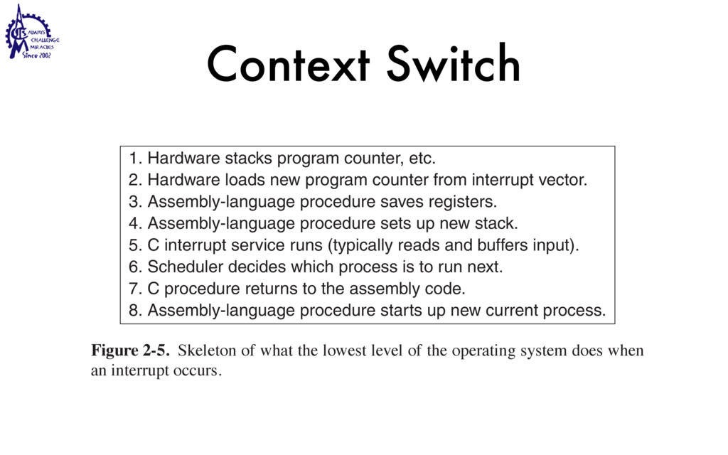
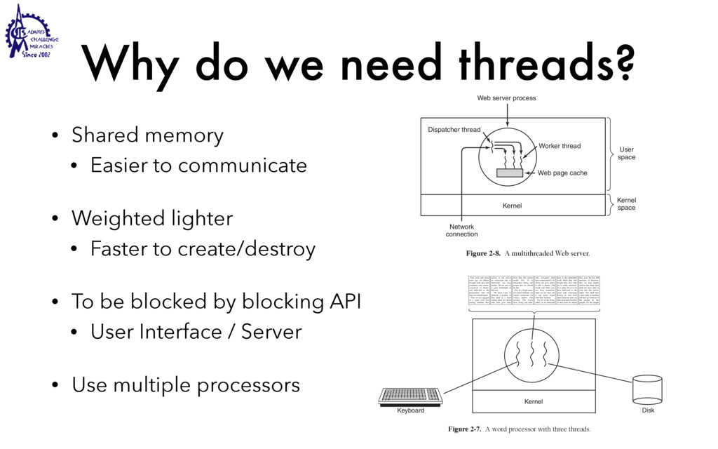
to communicate • Weighted lighter • Faster to create/destroy • To be blocked by blocking API • User Interface / Server • Use multiple processors SEC. 2.2 THREADS 99 Threads can help here. Suppose that the word processor is written as a two- threaded program. One thread interacts with the user and the other handles reformatting in the background. As soon as the sentence is deleted from page 1, the interactive thread tells the reformatting thread to reformat the whole book. Mean- while, the interactive thread continues to listen to the keyboard and mouse and re- sponds to simple commands like scrolling page 1 while the other thread is computing madly in the background. With a little luck, the reformatting will be completed before the user asks to see page 600, so it can be displayed instantly. While we are at it, why not add a third thread? Many word processors have a feature of automatically saving the entire file to disk every few minutes to protect the user against losing a day’s work in the event of a program crash, system crash, or power failure. The third thread can handle the disk backups without interfering with the other two. The situation with three threads is shown in Fig. 2-7. Kernel Keyboard Disk Four score and seven years ago, our fathers brought forth upon this continent a new nation: conceived in liberty, and dedicated to the proposition that all men are created equal. Now we are engaged in a great civil war testing whether that nation, or any nation so conceived and so dedicated, can long endure. We are met on a great battlefield of that war. We have come to dedicate a portion of that field as a final resting place for those who here gave their lives that this nation might live. It is altogether fitting and proper that we should do this. But, in a larger sense, we cannot dedicate, we cannot consecrate we cannot hallow this ground. The brave men, living and dead, who struggled here have consecrated it, far above our poor power to add or detract. The world will little note, nor long remember, what we say here, but it can never forget what they did here. It is for us the living, rather, to be dedicated here to the unfinished work which they who fought here have thus far so nobly advanced. It is rather for us to be here dedicated to the great task remaining before us, that from these honored dead we take increased devotion to that cause for which they gave the last full measure of devotion, that we here highly resolve that these dead shall not have died in vain that this nation, under God, shall have a new birth of freedom and that government of the people by the people, for the people Figure 2-7. A word processor with three threads. is called a cache and is used in many other contexts as well. We saw CPU caches in Chap. 1, for example. One way to organize the Web server is shown in Fig. 2-8(a). Here one thread, the dispatcher, reads incoming requests for work from the network. After examin- ing the request, it chooses an idle (i.e., blocked) worker thread and hands it the request, possibly by writing a pointer to the message into a special word associated with each thread. The dispatcher then wakes up the sleeping worker, moving it from blocked state to ready state. Dispatcher thread Worker thread Web page cache Kernel Network connection Web server process User space Kernel space Figure 2-8. A multithreaded Web server. When the worker wakes up, it checks to see if the request can be satisfied from the Web page cache, to which all threads have access. If not, it starts a read operation to get the page from the disk and blocks until the disk operation completes.

Not Everything Shared cooperate, not fight. In addition to sharing
an address space, all the threads can share the same set of open files, child processes, alarms, and signals, an so on, as shown in Fig. 2-12. Thus, the organization of Fig. 2-11(a) would be used when the hree processes are essentially unrelated, whereas Fig. 2-11(b) would be ap- propriate when the three threads are actually part of the same job and are actively and closely cooperating with each other. Per-process items Per-thread items Address space Program counter Global var iables Registers Open files Stack Child processes State Pending alarms Signals and signal handlers Accounting infor mation Figure 2-12. The first column lists some items shared by all threads in a process. The second one lists some items private to each thread. The items in the first column are process properties, not thread properties. For example, if one thread opens a file, that file is visible to the other threads in the process and they can read and write it. This is logical, since the process is the unit thread currently has the CPU and is active. In contrast, a blocked thread is for some event to unblock it. For example, when a thread performs a system read from the keyboard, it is blocked until input is typed. A thread can blo ing for some external event to happen or for some other thread to unblo ready thread is scheduled to run and will as soon as its turn comes up. T sitions between thread states are the same as those between process states illustrated in Fig. 2-2. It is important to realize that each thread has its own stack, as illus Fig. 2-13. Each thread’s stack contains one frame for each procedure ca not yet returned from. This frame contains the procedure’s local variables return address to use when the procedure call has finished. For example, dure X calls procedure Y and Y calls procedure Z, then while Z is execu frames for X, Y, and Z will all be on the stack. Each thread will generally ferent procedures and thus have a different execution history. This is w thread needs its own stack. Kernel Thread 3's stack Process Thread 3 Thread 1 Thread 2 Thread 1's stack Figure 2-13. Each thread has its own stack.

Thread Primitives a user-level threads package can be implemented on
an operating system that does not support threads. All operating systems used to fall into this category, and even now some still do. With this approach, threads are implemented by a library. All of these implementations have the same general structure, illustrated in Fig. 2-16(a). The threads run on top of a run-time system, which is a collection of procedures that manage threads. We hav e seen four of these already: pthread create, pthread exit, pthread join, and pthread yield, but usually there are more. Process Process Thread Thread Process table Process table Thread table Thread table Run-time system Kernel space User space Kernel Kernel Figure 2-16. (a) A user-level threads package. (b) A threads package managed by the kernel. When threads are managed in user space, each process needs its own private thread table to keep track of the threads in that process. This table is analogous to • create • exit • join • yield

in User Space vs Kernel • in User Space •
Coroutine • Fast • Require  non-blocking APIs • in Kernel • Safe to call   blocking APIs • Multiprocessors • Hybrid • goroutine in Golang a user-level threads package can be implemented on an operating system that does not support threads. All operating systems used to fall into this category, and even now some still do. With this approach, threads are implemented by a library. All of these implementations have the same general structure, illustrated in Fig. 2-16(a). The threads run on top of a run-time system, which is a collection of procedures that manage threads. We hav e seen four of these already: pthread create, pthread exit, pthread join, and pthread yield, but usually there are more. Process Process Thread Thread Process table Process table Thread table Thread table Run-time system Kernel space User space Kernel Kernel Figure 2-16. (a) A user-level threads package. (b) A threads package managed by the kernel. When threads are managed in user space, each process needs its own private thread table to keep track of the threads in that process. This table is analogous to

clone() in Linux • clone() • fork() / pthread_create() •
pid = clone(function, stack_ptr, sharing_ﬂags, arg); SEC. 10.3 PROCESSES IN LINUX 745 structure or shares it with the calling thread. Fig. 10-9 shows some of the items that can be shared or copied according to bits in sharing flags. Flag Meaning when set Meaning when cleared CLONE VM Create a new thread Create a new process CLONE FS Share umask, root, and wor king dirs Do not share them CLONE FILES Share the file descriptors Copy the file descriptors CLONE SIGHAND Share the signal handler table Copy the table CLONE PARENT New thread has same parent as the caller New thread’s parent is caller Figure 10-9. Bits in the sharing flags bitmap. The CLONE VM bit determines whether the virtual memory (i.e., address

Inter-Process Communication

Race Condition • Read-Modify-Write example: • y = x+1; •
x = y; • Critical Region • Program where the shared memory is accessed • Background • No two processes may be simultaneously inside their critical regions. • No assumptions may be made about speeds or the number of CPUs. • No process running outside its critical region may block any process. • No process should have to wait forever to enter its critical region.

Mutual Exclusion • Solutions • Disabling Interrupts • Peterson’s Algorithm
• Hardware atomic instruction • Can’t without hardware’s help, I suppose. • Mind compiler/hardware reordering

Disabling Interrupts • Not a good idea in user space
• But indeed used in kernel • Especially, before interrupt handlers are set up.

Peterson’s Algorithm • Don’t need atomic instructions • Wastes CPU
(as it busy-waits), unless it yield() flag[0] = false; flag[1] = false; int turn; flag[0] = true; turn = 1; while (flag[1] == true && turn == 1) ;// busy wait // critical section ... // end of critical section flag[0] = false; flag[1] = true; turn = 0; while (flag[0] == true && turn == 0) ; // busy wait // critical section ... // end of critical section flag[1] = false;

Hardware Atomic Instruction SEC. 2.3 INTERPROCESS COMMUNICATION 127 enter region:
TSL REGISTER,LOCK | copy lock to register and set lock to 1 CMP REGISTER,#0 | was lock zero? JNE enter region | if it was not zero, lock was set, so loop RET | retur n to caller; critical region entered leave region: MOVE LOCK,#0 | store a 0 in lock RET | retur n to caller Figure 2-25. Entering and leaving a critical region using the TSL instruction. An alternative instruction to TSL is XCHG, which exchanges the contents of two locations atomically, for example, a register and a memory word. The code is shown in Fig. 2-26, and, as can be seen, is essentially the same as the solution with TSL. All Intel x86 CPUs use XCHG instruction for low-level synchronization. enter region: MOVE REGISTER,#1 | put a 1 in the register XCHG REGISTER,LOCK | swap the contents of the register and lock var iable CMP REGISTER,#0 | was lock zero? JNE enter region | if it was non zero, lock was set, so loop RET | retur n to caller; critical region entered SEC. 2.3 INTERPROCESS COMMUNICATION 127 enter region: TSL REGISTER,LOCK | copy lock to register and set lock to 1 CMP REGISTER,#0 | was lock zero? JNE enter region | if it was not zero, lock was set, so loop RET | retur n to caller; critical region entered leave region: MOVE LOCK,#0 | store a 0 in lock RET | retur n to caller Figure 2-25. Entering and leaving a critical region using the TSL instruction. An alternative instruction to TSL is XCHG, which exchanges the contents of two locations atomically, for example, a register and a memory word. The code is shown in Fig. 2-26, and, as can be seen, is essentially the same as the solution with TSL. All Intel x86 CPUs use XCHG instruction for low-level synchronization. enter region: MOVE REGISTER,#1 | put a 1 in the register XCHG REGISTER,LOCK | swap the contents of the register and lock var iable CMP REGISTER,#0 | was lock zero? JNE enter region | if it was non zero, lock was set, so loop RET | retur n to caller; critical region entered leave region: MOVE LOCK,#0 | store a 0 in lock RET | retur n to caller Figure 2-26. Entering and leaving a critical region using the XCHG instruction.

Synchronization • Sleep / Wakeup: it yield() implicitly • Mutex:
lock(), unlock() • Condition Variable: wait(mutex), signal(), broadcast() • Semaphore: up(), down()

Condition Variables • Typical usage: • mutex.lock(); • cv.wait(mutex); •
do_something(); • mutex.unlock();

Condition Variables • Why does cv.wait(mutex) need a mutex passed
in? • cv.wait(mutex) atomically • unlock the mutex • wait on the condition • relook the mutex again • Otherwise may failed to wake up

Mutex vs Binary Semaphore • Mutex lock; • lock.lock(); •
enter_critical_region(); • lock.unlock(); • Semaphore sem = 1; • sem.down(); • enter_critical_region(); • sem.up();

Mutex vs Binary Semaphore • Mutex • ownership of the
resource • can be unlocked only by the one locked it • Semaphore • the number of the resource ref: https://www.zhihu.com/question/47704079

Mutex + Condition Variable • Avoid busy waiting • Mutex:
Protect the critical region • Condition Variable: Notify an event happens • Prefer mutex + condition variable to semaphore • Linus Torvalds on semaphores

Message Passing • Primitives • send(dest, msg) • recv(src, msg)
• Easy to scale out • Issues • Unreliable connection? • Performance • Security

Memory Barriers SEC. 2.3 INTERPROCESS COMMUNICATION 147 Barrier Barrier Barrier
A A A B B B C C D D D Time Time Time Process (a) (b) (c) C Figure 2-37. Use of a barrier. (a) Processes approaching a barrier. (b) All processes but one blocked at the barrier. (c) When the last process arrives at the barrier, all of them are let through. In Fig. 2-37(a) we see four processes approaching a barrier. What this means is that they are just computing and have not reached the end of the current phase yet. After a while, the first process finishes all the computing required of it during the first phase. It then executes the barr ier primitive, generally by calling a library pro- while (f == 0); // Memory fence required here print x; x = 42; // Memory fence required here f = 1;

Figure 43-1: A taxonomy of UNIX IPC facilities communication data
transfer message byte stream shared memory synchronization semaphore file lock fcntl()) flock()) signal pseudoterminal anonymous mapping

Producer-Consumer Pattern

Using Semaphores • Can’t work when there are multiple producers
and/or consumers semaphore fillCount = 0; semaphore emptyCount = BUFFER_SIZE; procedure producer() { while (true) { item = produceItem(); down(emptyCount); putItemIntoBuffer(item); up(fillCount); } } procedure consumer() { while (true) { down(fillCount); item = removeItemFromBuffer(); up(emptyCount); consumeItem(item); } } code: https://en.wikipedia.org/wiki/Producer%E2%80%93consumer_problem#Using_semaphores

Using Semaphores • Works well semaphore buffer_mutex = 1; semaphore
fillCount = 0; semaphore emptyCount = BUFFER_SIZE; procedure producer() { while (true) { item = produceItem(); down(emptyCount); down(buffer_mutex); putItemIntoBuffer(item); up(buffer_mutex); up(fillCount); } } procedure consumer() { while (true) { down(fillCount); down(buffer_mutex); item = removeItemFromBuffer(); up(buffer_mutex); up(emptyCount); consumeItem(item); } } code: https://en.wikipedia.org/wiki/Producer%E2%80%93consumer_problem#Using_semaphores

Using Mutex + Condition Variable • Works well code: Modern
Operating Systems 4th, Figure 2-32 138 PROCESSES AND THREADS CHAP. 2 #include <stdio.h> #include <pthread.h> #define MAX 1000000000 /* how many numbers to produce */ pthread mutex t the mutex; pthread cond t condc, condp; /* used for signaling */ int buffer = 0; /* buffer used between producer and consumer */ void *producer(void *ptr) /* produce data */ { int i; for (i= 1; i <= MAX; i++) { pthread mutex lock(&the mutex); /* get exclusive access to buffer */ while (buffer != 0) pthread cond wait(&condp, &the mutex); buffer = i; /* put item in buffer */ pthread cond signal(&condc); /* wake up consumer */ pthread mutex unlock(&the mutex); /* release access to buffer */ } pthread exit(0); } void *consumer(void *ptr) /* consume data */ { int i; for (i = 1; i <= MAX; i++) { pthread mutex lock(&the mutex); /* get exclusive access to buffer */ while (buffer ==0 ) pthread cond wait(&condc, &the mutex); buffer = 0; /* take item out of buffer */ pthread cond signal(&condp); /* wake up producer */ pthread mutex unlock(&the mutex); /* release access to buffer */ } pthread exit(0); } int main(int argc, char **argv)

Using Message Passing • Works well code: Modern Operating Systems
4th, Figure 2-32 146 PROCESSES AND THREADS CHAP. 2 #define N 100 /* number of slots in the buffer */ void producer(void) { int item; message m; /* message buffer */ while (TRUE) { item = produce item( ); /* generate something to put in buffer */ receive(consumer, &m); /* wait for an empty to arrive */ build message(&m, item); /* constr uct a message to send */ send(consumer, &m); /* send item to consumer */ } } void consumer(void) { int item, i; message m; for (i = 0; i < N; i++) send(producer, &m); /* send N empties */ while (TRUE) { receive(producer, &m); /* get message containing item */ item = extract item(&m); /* extract item from message */ send(producer, &m); /* send back empty reply */ consume item(item); /* do something with the item */ } }

Dining Philosophers Problem

Using Semaphores { while (TRUE) { /* repeat forever */
think( ); /* philosopher is thinking */ take forks(i); /* acquire two for ks or block */ eat( ); /* yum-yum, spaghetti */ put forks(i); /* put both for ks back on table */ } } void take forks(int i) /* i: philosopher number, from 0 to N−1 */ { down(&mutex); /* enter critical region */ state[i] = HUNGRY; /* record fact that philosopher i is hungry */ test(i); /* tr y to acquire 2 for ks */ up(&mutex); /* exit critical region */ down(&s[i]); /* block if for ks were not acquired */ } void put forks(i) /* i: philosopher number, from 0 to N−1 */ { down(&mutex); /* enter critical region */ state[i] = THINKING; /* philosopher has finished eating */ test(LEFT); /* see if left neighbor can now eat */ test(RIGHT); /* see if right neighbor can now eat */ up(&mutex); /* exit critical region */ } void test(i) /* i: philosopher number, from 0 to N−1 */ { if (state[i] == HUNGRY && state[LEFT] != EATING && state[RIGHT] != EATING) { state[i] = EATING; up(&s[i]); } } Figure 2-47. A solution to the dining philosophers problem. 170 PROCESSES AND THREADS CHAP. 2 #define N 5 /* number of philosophers */ #define LEFT (i+N−1)%N /* number of i’s left neighbor */ #define RIGHT (i+1)%N /* number of i’s right neighbor */ #define THINKING 0 /* philosopher is thinking */ #define HUNGRY 1 /* philosopher is trying to get for ks */ #define EATING 2 /* philosopher is eating */ typedef int semaphore; /* semaphores are a special kind of int */ int state[N]; /* array to keep track of everyone’s state */ semaphore mutex = 1; /* mutual exclusion for critical regions */ semaphore s[N]; /* one semaphore per philosopher */ void philosopher(int i) /* i: philosopher number, from 0 to N−1 */ { while (TRUE) { /* repeat forever */ think( ); /* philosopher is thinking */ take forks(i); /* acquire two for ks or block */ eat( ); /* yum-yum, spaghetti */ put forks(i); /* put both for ks back on table */ } } void take forks(int i) /* i: philosopher number, from 0 to N−1 */ { down(&mutex); /* enter critical region */ state[i] = HUNGRY; /* record fact that philosopher i is hungry */ test(i); /* tr y to acquire 2 for ks */ up(&mutex); /* exit critical region */ down(&s[i]); / block if for ks were not acquired /

Scheduling

Goals Scheduling Algorithm Goals In order to design a scheduling
algorithm, it is necessary to have some idea of what a good algorithm should do. Some goals depend on the environment (batch, interactive, or real time), but some are desirable in all cases. Some goals are listed in Fig. 2-40. We will discuss these in turn below. All systems Fair ness - giving each process a fair share of the CPU Policy enforcement - seeing that stated policy is carried out Balance - keeping all parts of the system busy Batch systems Throughput - maximize jobs per hour Turnaround time - minimize time between submission and termination CPU utilization - keep the CPU busy all the time Interactive systems Response time - respond to requests quickly Propor tionality - meet users’ expectations Real-time systems Meeting deadlines - avoid losing data Predictability - avoid quality degradation in multimedia systems Figure 2-40. Some goals of the scheduling algorithm under different circumstances. Under all circumstances, fairness is important. Comparable processes should

Algorithms for Batch Systems • First-Come, First-Served • Consider: CPU-bound
ﬁrst, then lots of I/O-bound • Shortest Job First • minimize turnaround • optimal only when all the jobs are available simultaneously • run time has to be known in advance • Shortest Remaining Time Next

Algorithms for Interactive Systems • Round-Robin • Priority Scheduling •
Multiple Queues • High priority tasks tend to run fast • Whenever a process used up all the quanta allocated to it, it was moved down one class • Shortest Process Next • Estimate the running time on the ﬂy SEC. 2.4 SCHEDULING Priority 4 Priority 3 Priority 2 Priority 1 Queue headers Runnable processes (Highest priority) (Lowest priority) Figure 2-43. A scheduling algorithm with four priority classes. Multiple Queues One of the earliest priority schedulers was in CTSS, the M.I.T. TimeSharing System that ran on the IBM 7094 (Corbato ´ et al., 1962) the problem that process switching was slow because the 7094 could h process in memory. Each switch meant swapping the current process reading in a new one from disk. The CTSS designers quickly realize more efficient to give CPU-bound processes a large quantum once in a er than giving them small quanta frequently (to reduce swapping). O hand, giving all processes a large quantum would mean poor response have already seen. Their solution was to set up priority classes. Proc highest class were run for one quantum. Processes in the next-highes run for two quanta. Processes in the next one were run for four quanta

Algorithms for Interactive Systems • Guaranteed Scheduling • Each process
receive about 1/n of the CPU power • Lottery Scheduling • Weighted • Randomly choose one • Fair-Share Scheduling • Each user receive about 1/n of the CPU power

Scheduling in Real-Time Systems • Hard real-time systems • Soft
real-time systems: tolerant missing an occasional deadline • Schedulable • period Pi • requires Ci sec of CPU time • sum(Ci / Pi) ≤ 1

Mechanism and Policy • Separate scheduling mechanism from scheduling policy
• Mechanism: scheduling algorithm is parameterized in some way • Policy: parameters can be ﬁlled in by user processes.

Thread Scheduling • User-level Thread • Kernel-level Thread

Deadlocks

Conditions • Mutual exclusion condition. • Each resource is either
currently assigned to exactly one process or is available. • Hold-and-wait condition. • Processes currently holding resources that were granted earlier can request new resources. • No-preemption condition. • Resources previously granted cannot be forcibly taken away from a process. They must be explicitly released by the process holding them. • Circular wait condition. • There must be a circular list of two or more processes, each of which is waiting for a resource held by the next member of the chain.

Deadlock Example • Avoid deadlock • Attack circular wait condition
• Ensure partial order SEC. 6.2 INTRODUCTION TO DEADLOCKS 439 typedef int semaphore; semaphore resource 1; semaphore resource 1; semaphore resource 2; semaphore resource 2; void process A(void) { void process A(void) { down(&resource 1); down(&resource 1); down(&resource 2); down(&resource 2); use both resources( ); use both resources( ); up(&resource 2); up(&resource 2); up(&resource 1); up(&resource 1); } } void process B(void) { void process B(void) { down(&resource 1); down(&resource 2); down(&resource 2); down(&resource 1); use both resources( ); use both resources( ); up(&resource 2); up(&resource 1); up(&resource 1); up(&resource 2); } } (a) (b) Figure 6-2. (a) Deadlock-free code. (b) Code with a potential deadlock.

Memory Management

Memory Abstraction

No Abstraction • Need relocation • Dangerous operating system is
in high memory and thus not shown. 0 4 8 12 16 20 24 28 0 4 8 12 16 20 24 28 (a) (b) 0 4 8 12 16 20 24 28 ADD JMP 24 MOV (c) 16384 16388 16392 16396 16400 16404 16408 16412 ADD JMP 24 MOV 0 16380 JMP 28 CMP 0 16380 . . . . . . . . . 16380 . . . JMP 28 CMP 0 0 32764 Figure 3-2. Illustration of the relocation problem. (a) A 16-KB program. (b) Another 16-KB program. (c) The two programs loaded consecutively into memory.

Address Spaces • Dynamic relocation • Base + Limit register
• Memory overload • Swapping • Virtual Memory 188 MEMORY MANAGEMENT CHA 0 4 8 12 16 20 24 28 (c) ADD JMP 24 MOV JMP 28 CMP . . . 0 . . . 0 16384 16388 16392 16396 16400 16404 16408 16412 16380 32764 16384 16384 Base register Limit register Figure 3-3. Base and limit registers can be used to give each process a separate address space.

Address Spaces • Need to deal with holes process A
is in memory. Then processes B and C are created or swapped in from disk. In Fig. 3-4(d) A is swapped out to disk. Then D comes in and B goes out. Finally A comes in again. Since A is now at a different location, addresses con- tained in it must be relocated, either by software when it is swapped in or (more likely) by hardware during program execution. For example, base and limit registers would work fine here. (a) Operating system A (b) Operating system A B (c) Operating system A B C (d) Time Operating system B C (e) D Operating system B C (f) D Operating system C (g) D Operating system A C Figure 3-4. Memory allocation changes as processes come into memory and leave it. The shaded regions are unused memory. When swapping creates multiple holes in memory, it is possible to combine them all into one big one by moving all the processes downward as far as possible. This technique is known as memory compaction. It is usually not done because it requires a lot of CPU time. For example, on a 16-GB machine that can copy 8 bytes in 8 nsec, it would take about 16 sec to compact all of memory.

Manage Free List • Allocation Units • Bitmap • Simple
• Space-efﬁcient • Linked List • More balanced on all kinds of operations Memory Management with Bitmaps With a bitmap, memory is divided into allocation units as small as a few words and as large as several kilobytes. Corresponding to each allocation unit is a bit in the bitmap, which is 0 if the unit is free and 1 if it is occupied (or vice versa). Fig- ure 3-6 shows part of memory and the corresponding bitmap. (a) (b) (c) A B C D E 8 16 24 Hole Starts at 18 Length 2 Process P 0 5 H 5 3 P 8 6 P 14 4 H 18 2 P 20 6 P 26 3 H 29 3 X 1 1 1 1 1 0 0 0 1 1 1 1 1 1 1 1 1 1 0 0 1 1 1 1 1 1 1 1 1 0 0 0 Figure 3-6. (a) A part of memory with fiv e processes and three holes. The tick marks show the memory allocation units. The shaded regions (0 in the bitmap) are free. (b) The corresponding bitmap. (c) The same information as a list. The size of the allocation unit is an important design issue. The smaller the allocation unit, the larger the bitmap. However, even with an allocation unit as small as 4 bytes, 32 bits of memory will require only 1 bit of the map. A memory of 32n

Virtual Memory

Virtual Memory SEC. 3.3 VIRTUAL MEMORY Virtual address space Physical
memory address 60K–64K 56K–60K 52K–56K 48K–52K 44K–48K 40K–44K 36K–40K 32K–36K 28K–32K 24K–28K 20K–24K 16K–20K 12K–16K 8K–12K 4K–8K 0K–4K 28K–32K 24K–28K 20K–24K 16K–20K 12K–16K 8K–12K 4K–8K 0K–4K Virtual page Page frame X X X X 7 X 5 X X X 3 4 0 6 1 2 left image: https://en.wikipedia.org/wiki/File:X86_Paging_4K.svg

Speeding Up Using TLB image: https://en.wikipedia.org/wiki/File:Page_table_actions.svg

Page Tables for Large Memories • Multilevel Page Tables •
Linux: four-level page tables • Inverted Page Tables • physics address => virtual address • maybe use hash SEC. 10.4 MEMORY MANAGEMENT IN LINUX 761 Global directory Upper directory Middle directory Page Offset Page Page table Page middle directory Page upper directory Page global directory Virtual address Figure 10-16. Linux uses four-level page tables.

Page Replacement Algorithms • The Optimal Page Replacement Algorithm •
Page with the latest next reference time should be removed • Only theoretic value; Not realizable • The Not Recently Used Page Replacement Algorithm • R/M bits; Periodically clears R bits; • Class 0: not referenced, not modiﬁed; …; Class 3: referenced, modiﬁed. • Approximation to the optimal one

Page Replacement Algorithms • The First-In, First-Out Page Replacement Algorithm
• the oldest page may still be useful; rarely used • The Second-Chance Page Replacement Algorithm • FIFO + R bits • If the list head has R bit, clear and move to tail. • The Clock Page Replacement Algorithm • Use circular list 212 MEMORY MANAGEMENT CHAP. 3 3.4.4 The Second-Chance Page Replacement Algorithm A simple modification to FIFO that avoids the problem of throwing out a heavily used page is to inspect the R bit of the oldest page. If it is 0, the page is both old and unused, so it is replaced immediately. If the R bit is 1, the bit is cleared, the page is put onto the end of the list of pages, and its load time is updated as though it had just arrived in memory. Then the search continues. The operation of this algorithm, called second chance, is shown in Fig. 3-15. In Fig. 3-15(a) we see pages A through H kept on a linked list and sorted by the time they arrived in memory. (a) Page loaded first Most recently loaded page 0 A 3 B 7 C 8 D 12 E 14 F 15 G 18 H A is treated like a newly loaded page 3 B 7 C 8 D 12 E 14 F 15 G 18 H 20 A 212 MEMORY MANAGEMENT CHAP. 3 3.4.4 The Second-Chance Page Replacement Algorithm A simple modification to FIFO that avoids the problem of throwing out a heavily used page is to inspect the R bit of the oldest page. If it is 0, the page is both old and unused, so it is replaced immediately. If the R bit is 1, the bit is cleared, the page is put onto the end of the list of pages, and its load time is updated as though it had just arrived in memory. Then the search continues. The operation of this algorithm, called second chance, is shown in Fig. 3-15. In Fig. 3-15(a) we see pages A through H kept on a linked list and sorted by the time they arrived in memory. (a) Page loaded first Most recently loaded page 0 A 3 B 7 C 8 D 12 E 14 F 15 G 18 H (b) A is treated like a newly loaded page 3 B 7 C 8 D 12 E 14 F 15 G 18 H 20 A Figure 3-15. Operation of second chance. (a) Pages sorted in FIFO order. (b) Page list if a page fault occurs at time 20 and A has its R bit set. The numbers above the pages are their load times. Suppose that a page fault occurs at time 20. The oldest page is A, which arrived at time 0, when the process started. If A has the R bit cleared, it is evicted from SEC. 3.4 PA GE REPLACEMENT ALGORITHMS When a page fault occurs, the page the hand is pointing to is inspected. The action taken depends on the R bit: R = 0: Evict the page R = 1: Clear R and advance hand A B C D E F G H I J K L Figure 3-16. The clock page replacement algorithm. When a page fault occurs, the page being pointed to by the hand is ins If its R bit is 0, the page is evicted, the new page is inserted into the cloc place, and the hand is advanced one position. If R is 1, it is cleared and the advanced to the next page. This process is repeated until a page is foun R = 0. Not surprisingly, this algorithm is called clock. 3.4.6 The Least Recently Used (LRU) Page Replacement Algorith A good approximation to the optimal algorithm is based on the obse that pages that have been heavily used in the last few instructions will proba heavily used again soon. Conversely, pages that have not been used for ag probably remain unused for a long time. This idea suggests a realizable alg when a page fault occurs, throw out the page that has been unused for the

Page Replacement Algorithms • The Least Recently Used Page Replacement
Algorithm • Hard to track • The Not Frequently Used Page Replacement Algorithm • Link List + Hash Table ?? • Aging??

Page Replacement Algorithms • The Working Set Page Replacement Algorithm
• The WSClock Page Replacement Algorithm

Buddy Allocator • Linux uses Buddy + Slab Fig. 10-17(a).
When a request for memory comes in, it is first rounded up to a power of 2, say eight pages. The full memory chunk is then divided in half, as shown in (b). Since each of these pieces is still too large, the lower piece is divided in half again (c) and again (d). Now we hav e a chunk of the correct size, so it is allocated to the caller, as shown shaded in (d). (a) 64 (b) 32 32 (d) 32 8 8 16 (e) 16 8 8 32 (f) 8 8 8 32 8 (g) 8 4 8 8 32 (h) 4 8 8 8 32 (i) 16 4 4 8 32 (c) 16 16 32 4 4 Figure 10-17. Operation of the buddy algorithm. Now suppose that a second request comes in for eight pages. This can be satisfied directly now (e). At this point a third request comes in for four pages. The smallest available chunk is split (f) and half of it is claimed (g). Next, the second

Page Fault Handling 1. The hardware traps to the kernel,
saving the program counter on the stack. On most machines, some information about the state of the current instruction is saved in special CPU registers. 2. An assembly-code routine is started to save the general registers and other volatile information, to keep the operating system from destroying it. This routine calls the operating system as a procedure. 3. The operating system discovers that a page fault has occurred, and tries to discover which virtual page is needed. Often one of the hardware registers contains this information. If not, the operating system must retrieve the program counter, fetch the instruction, and parse it in software to ﬁgure out what it was doing when the fault hit. text: Modern Operating Systems 4th, Section 3.6.2

Page Fault Handling 4. Once the virtual address that caused
the fault is known, the system checks to see if this address is valid and the protection is consistent with the access. If not, the process is sent a signal or killed. If the address is valid and no protection fault has occurred, the system checks to see if a page frame is free. If no frames are free, the page replacement algorithm is run to select a victim. 5. If the page frame selected is dirty, the page is scheduled for transfer to the disk, and a context switch takes place, suspending the faulting process and letting another one run until the disk transfer has completed. In any event, the frame is marked as busy to prevent it from being used for another purpose. 6. As soon as the page frame is clean (either immediately or after it is written to disk), the operating system looks up the disk address where the needed page is, and schedules a disk operation to bring it in. While the page is being loaded, the faulting process is still suspended and another user process is run, if one is available. text: Modern Operating Systems 4th, Section 3.6.2

Page Fault Handling 7. When the disk interrupt indicates that
the page has arrived, the page tables are updated to reﬂect its position, and the frame is marked as being in the normal state. 8. The faulting instruction is backed up to the state it had when it began and the program counter is reset to point to that instruction. 9. The faulting process is scheduled, and the operating system returns to the (assembly-language) routine that called it. 10.This routine reloads the registers and other state information and returns to user space to continue execution, as if no fault had occurred. text: Modern Operating Systems 4th, Section 3.6.2

Policy and Mechanism • For example: • A low-level MMU
handler. • A page fault handler that is part of the kernel. • An external pager running in user space. • Policy: • Page replacement algorithm 240 MEMORY MANAGEMENT CHAP Disk Main memory External pager Fault handler User process MMU handler 1. Page fault 6. Map page in 5. Here is page User space Kernel space 2. Needed page 4. Page arrives 3. Request page Figure 3-29. Page fault handling with an external pager.

Segmentation

Segmentation can grow or shrink independently without affecting each other.
If a stack in a cer- tain segment needs more address space to grow, it can have it, because there is nothing else in its address space to bump into. Of course, a segment can fill up, but segments are usually very large, so this occurrence is rare. To specify an address in this segmented or two-dimensional memory, the program must supply a two-part address, a segment number, and an address within the segment. Figure 3-31 illus- trates a segmented memory being used for the compiler tables discussed earlier. Five independent segments are shown here. Symbol table Source text Constants Parse tree Call stack Segment 0 Segment 1 Segment 2 Segment 3 Segment 4 20K 16K 12K 8K 4K 0K 12K 8K 4K 0K 0K 16K 12K 8K 4K 0K 12K 8K 4K 0K Figure 3-31. A segmented memory allows each table to grow or shrink independently of the other tables. We emphasize here that a segment is a logical entity, which the programmer is aw are of and uses as a logical entity. A segment might contain a procedure, or an array, or a stack, or a collection of scalar variables, but usually it does not contain a mixture of different types. A segmented memory has other advantages besides simplifying the handling of data structures that are growing or shrinking. If each procedure occupies a sepa- The hardware then uses the Limit field to check if the offset is beyon of the segment, in which case a trap also occurs. Logically, there should be field in the descriptor giving the size of the segment, but only 20 bits are a so a different scheme is used. If the Gbit (Granularity) field is 0, the Lim the exact segment size, up to 1 MB. If it is 1, the Limit field gives the segm in pages instead of bytes. With a page size of 4 KB, 20 bits are enough ments up to 232 bytes. Assuming that the segment is in memory and the offset is in range then adds the 32-bit Base field in the descriptor to the offset to form what a linear address, as shown in Fig. 3-40. The Base field is broken up i pieces and spread all over the descriptor for compatibility with the 286, the Base is only 24 bits. In effect, the Base field allows each segment to s arbitrary place within the 32-bit linear address space. Descriptor Base address Limit Other fields 32-Bit linear address + + Selector Offset Figure 3-40. Conversion of a (selector, offset) pair to a linear address.

File Systems

Why File Systems? • Hard drive primitives: • Read /
Write Block k • But • How do you ﬁnd information? • How do you keep one user from reading another user’s data? • How do you know which blocks are free? • …

File Operations • create • delete • open • close
• read • write • append • seek • get attributes • set attributes • rename

Directory Operations • create • delete • opendir • closedir
• readdir • rename • link • unlink

Shared Files / Directories • Hard Link: reference counting •
Symbolic Link: a special ﬁle

File System Layout Other than starting with a boot block,
the layout of a disk partition varies a lot from file system to file system. Often the file system will contain some of the items shown in Fig. 4-9. The first one is the superblock. It contains all the key parameters about the file system and is read into memory when the computer is booted or the file system is first touched. Typical information in the superblock includes a magic number to identify the file-system type, the number of blocks in the file system, and other key administrative information. Entire disk Disk partition Partition table Files and directories Root dir I-nodes Superblock Free space mgmt Boot block MBR Figure 4-9. A possible file-system layout. Next might come information about free blocks in the file system, for example in the form of a bitmap or a list of pointers. This might be followed by the i-nodes, an array of data structures, one per file, telling all about the file. After that might come the root directory, which contains the top of the file-system tree. Finally, the remainder of the disk contains all the other directories and files. 4.3.2 Implementing Files Probably the most important issue in implementing file storage is keeping track of which disk blocks go with which file. Various methods are used in different operating systems. In this section, we will examine a few of them. ext2. The first Linux release used the MINIX 1 file system and was limi short file names and 64-MB file sizes. The MINIX 1 file system was eventua placed by the first extended file system, ext, which permitted both long names and larger file sizes. Due to its performance inefficiencies, ext was re by its successor, ext2, which is still in widespread use. An ext2 Linux disk partition contains a file system with the layout sho Fig. 10-31. Block 0 is not used by Linux and contains code to boot the com Following block 0, the disk partition is divided into groups of blocks, irresp of where the disk cylinder boundaries fall. Each group is organized as follow The first block is the superblock. It contains information about the lay the file system, including the number of i-nodes, the number of disk block the start of the list of free disk blocks (typically a few hundred entries). comes the group descriptor, which contains information about the location bitmaps, the number of free blocks and i-nodes in the group, and the number rectories in the group. This information is important since ext2 attempts to directories evenly over the disk. Boot Block group 0 Super– Group block descriptor Block group 1 Block bitmap Data blocks I–node bitmap I–nodes Block group 2 Block group 3 Block group 4 Figure 10-31. Disk layout of the Linux ext2 file system.

Contiguous Allocation • High performance • Fragment • Useful for
readonly ﬁle systems the end of file A. Note that each file begins at the start of a new block, so that if file A was really 3½ blocks, some space is wasted at the end of the last block. In the figure, a total of seven files are shown, each one starting at the block following the end of the previous one. Shading is used just to make it easier to tell the files apart. It has no actual significance in terms of storage. … File A (4 blocks) File C (6 blocks) File B (3 blocks) File D (5 blocks) File F (6 blocks) File E (12 blocks) File G (3 blocks) (a) … (File A) (File C) File B 5 Free blocks 6 Free blocks (File E) (File G) (b) Figure 4-10. (a) Contiguous allocation of disk space for seven files. (b) The state of the disk after files D and F have been removed. Contiguous disk-space allocation has two significant advantages. First, it is simple to implement because keeping track of where a file’s blocks are is reduced to remembering two numbers: the disk address of the first block and the number of blocks in the file. Given the number of the first block, the number of any other

Linked List Allocation • Slow random access • Data block
size is no longer a power of two SEC. 4.3 FILE-SYSTEM IMPLEMENTATION File A Physical block Physical block 4 0 7 2 10 12 File block 0 File block 1 File block 2 File block 3 File block 4 File B 0 6 3 11 14 File block 0 File block 1 File block 2 File block 3 Figure 4-11. Storing a file as a linked list of disk blocks. Unlike contiguous allocation, every disk block can be used in this meth

File Allocation Table • Keep the linked list in memory
as a table • Data block size is a power of two • The table is in memory, thus faster to follow the link. • Costs memory. Don’t scale well. 286 FILE SYSTEMS C Physical block File A starts here File B starts here Unused block 0 1 2 3 4 5 6 7 8 9 10 11 12 13 14 15 10 11 7 3 2 12 14 -1 -1 Figure 4-12. Linked-list allocation using a file-allocation table in main memory.

I-nodes SEC. 4.5 EXAMPLE FILE SYSTEMS 325 I-node Attributes Disk
addresses Single indirect block Double indirect block Triple indirect block Addresses of data blocks Figure 4-33. A UNIX i-node. an i-node from its number is straightforward, since each one has a fixed location on the disk. From this i-node, the system locates the directory for /usr and looks up antage of this scheme over linked files using an in-memory table is that eed be in memory only when the corresponding file is open. If each i- ies n bytes and a maximum of k files may be open at once, the total cupied by the array holding the i-nodes for the open files is only kn this much space need be reserved in advance. File Attributes Address of disk block 0 Address of disk block 1 Address of disk block 2 Address of disk block 3 Address of disk block 4 Address of disk block 5 Address of disk block 6 Address of disk block 7 Address of block of pointers Disk block containing additional disk addresses Figure 4-13. An example i-node. ay is usually far smaller than the space occupied by the file table de-

I-nodes 326 FILE SYSTEMS CHAP. 4 Root directory I-node 6
is for /usr Block 132 is /usr directory I-node 26 is for /usr/ast Block 406 is /usr/ast directory Looking up usr yields i-node 6 I-node 6 says that /usr is in block 132 /usr/ast is i-node 26 /usr/ast/mbox is i-node 60 I-node 26 says that /usr/ast is in block 406 1 1 4 7 14 9 6 8 . .. bin dev lib etc usr tmp 6 1 19 30 51 26 45 dick erik jim ast bal 26 6 64 92 60 81 17 grants books mbox minix src Mode size times 132 Mode size times 406 Figure 4-34. The steps in looking up /usr/ast/mbox.

Journaling File Systems • To perform an operation • Write
a log entry listing all actions to be completed • Ensure the log is written to disk • Do all kinds of actions • Erase the log entry • The logged actions must be idempotent

Virtual File Systems SEC. 4.3 FILE-SYSTEM IMPLEMENTATION 299 are shown
in Fig. 4-19. Starting with the caller’s process number and the file descriptor, successively the v-node, read function pointer, and access function within the concrete file system are located. . . . Process table 0 File descriptors . . . V-nodes open read write Function pointers . . . 2 4 VFS Read function FS 1 Call from VFS into FS 1 Figure 4-19. A simplified view of the data structures and code used by the VFS and concrete file system to do a read.

Virtual File Systems wide area network if the server is
far from the client. For simplicity we will speak of clients and servers as though they were on distinct machines, but in fact, NFS allows every machine to be both a client and a server at the same time. Each NFS server exports one or more of its directories for access by remote clients. When a directory is made available, so are all of its subdirectories, so actually entire directory trees are normally exported as a unit. The list of directories a server exports is maintained in a file, often /etc/exports, so these directories can be exported automatically whenever the server is booted. Clients access exported directories by mounting them. When a client mounts a (remote) directory, it becomes part of its directory hierarchy, as shown in Fig. 10-35. Client 1 Client 2 Server 1 Server 2 / /usr /usr/ast /usr/ast/work /bin /bin cat cp Is mv sh a b c d e /proj2 /proj1 /projects /mnt /bin Mount / Figure 10-35. Examples of remote mounted file systems. Directories are shown as squares and files as circles. In this example, client 1 has mounted the bin directory of server 1 on its own bin directory, so it can now refer to the shell as /bin/sh and get the shell on server 1. Diskless workstations often have only a skeleton file system (in RAM) and get all their files from remote servers like this. Similarly, client 1 has mounted server 796 CASE STUDY 1: UNIX, LINUX, AND ANDROID CHAP. 10 Client kernel Server kernel System call layer Buffer cache Buffer cache Virtual file system layer Virtual file system layer Local FS 1 Local FS 1 Local FS 2 Local FS 2 NFS client NFS server Driver Driver Driver Driver Message to server Message from client Local disks Local disks V- node Figure 10-36. The NFS layer structure file system and i-node are recorded because modern Linux systems can support multiple file systems (e.g., ext2fs, /proc, FAT , etc.). Although VFS was invented to support NFS, most modern Linux systems now support it as an integral part of the operating system, even if NFS is not used.

Operating Systems Final Exam Review (ACM2014)

Operating Systems Final Exam Review (ACM2014)

More Decks by Lequn Chen

Featured

Transcript