Character Networks and Book Genre Classification

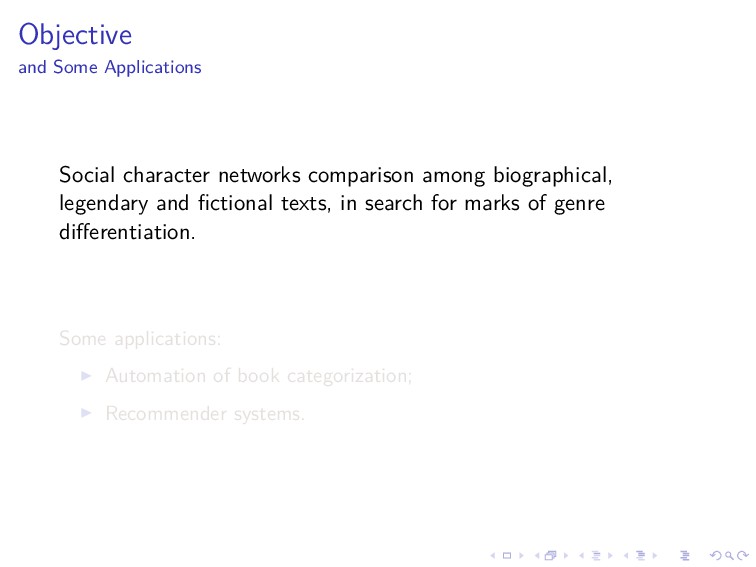
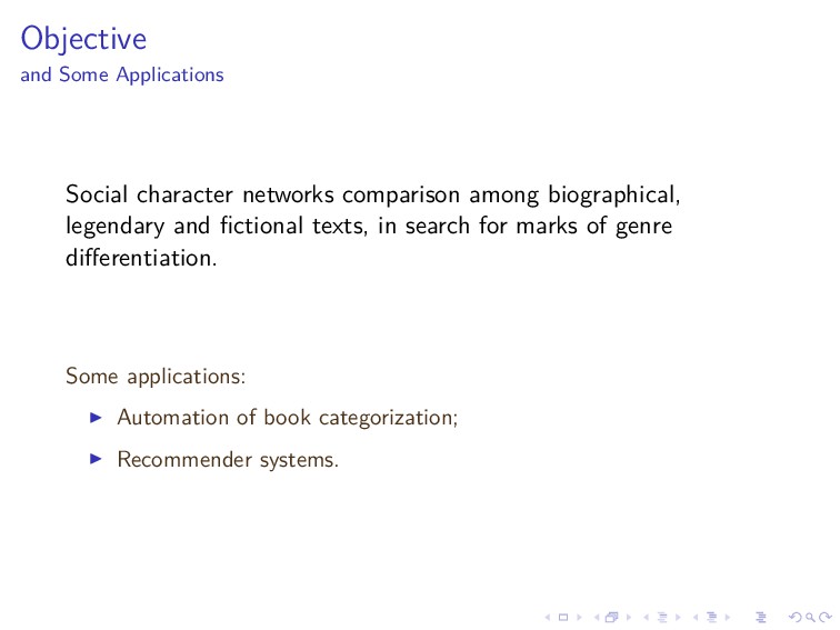
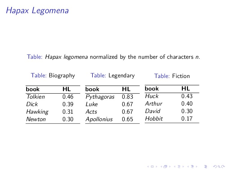
We compared the social character networks of biographical, legendary
and fictional texts, in search for marks of genre differentiation.
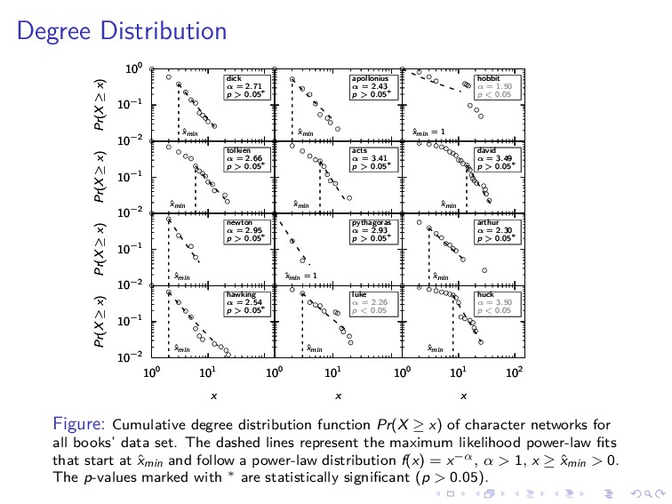
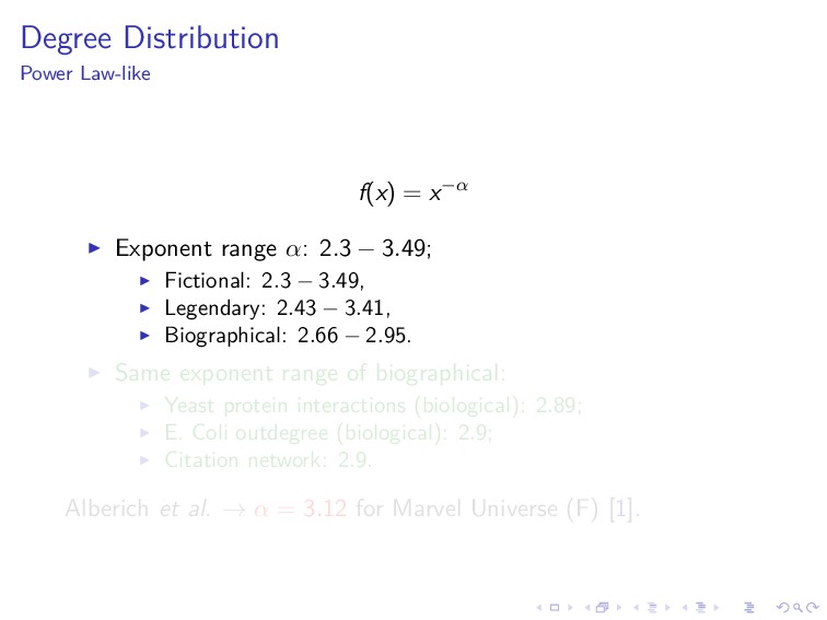
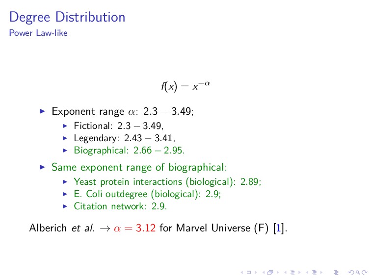
We examined the degree distribution of character appearance and
found a power-law-like distribution that does not depend on the
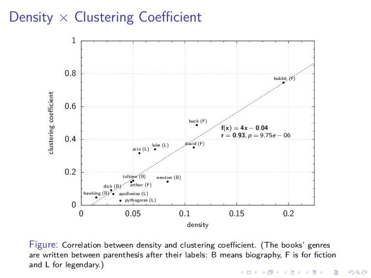
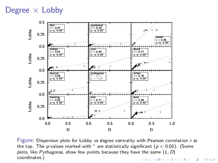
literary genre. We also analyzed local and global complex networks
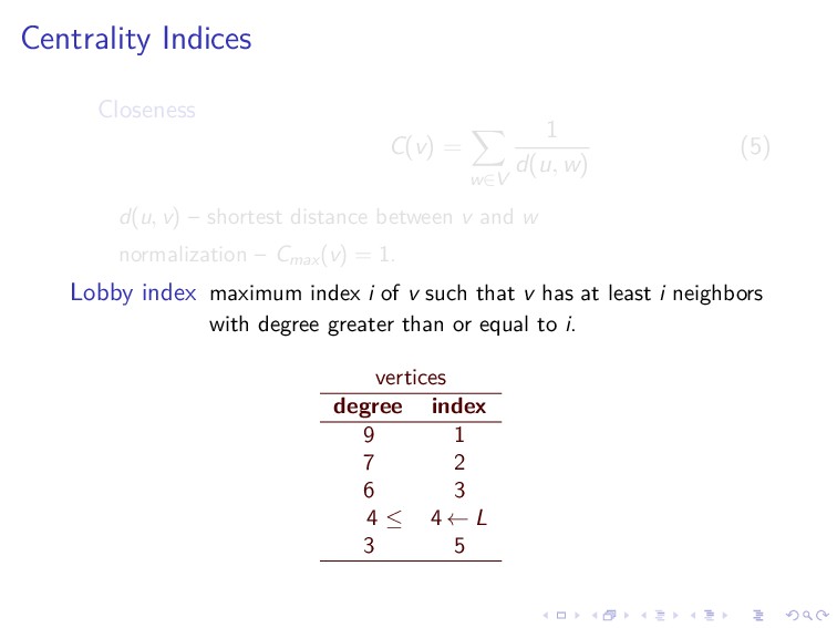
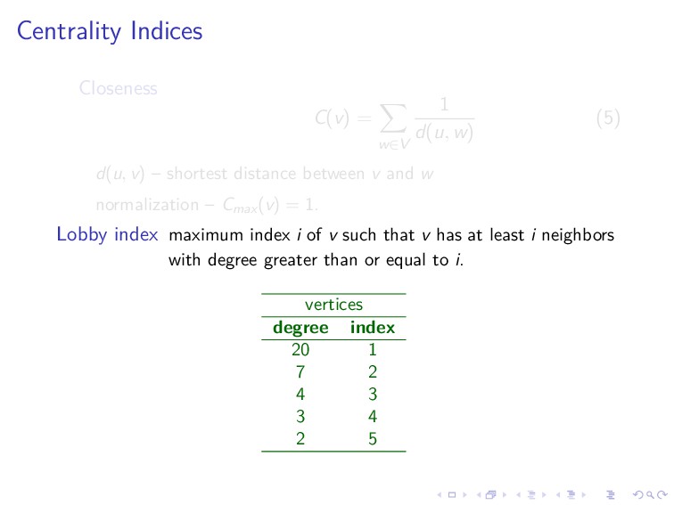
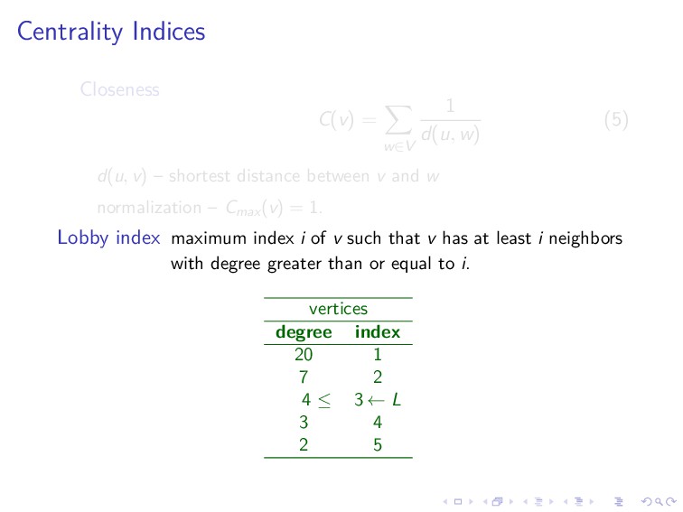
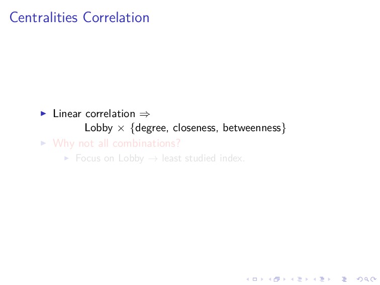
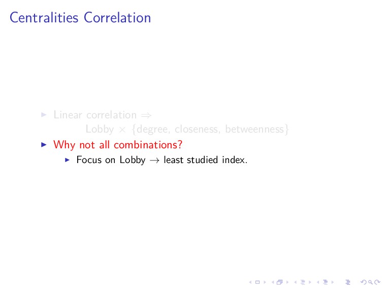
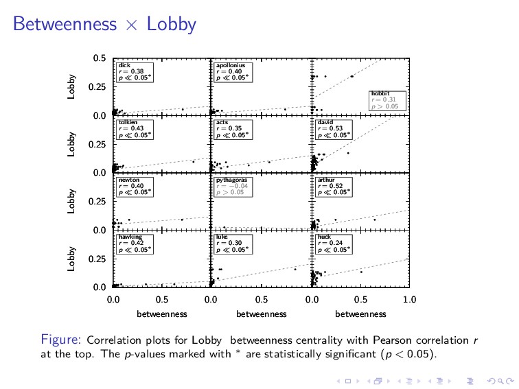
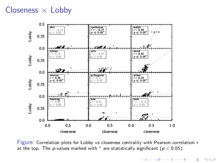
measures, in particular, correlation plots between the recently
introduced Lobby index and degree, betweenness and closeness
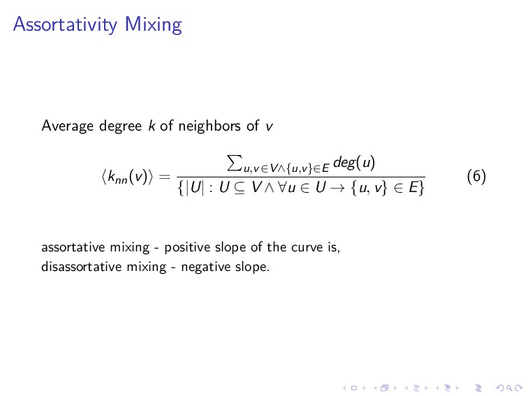
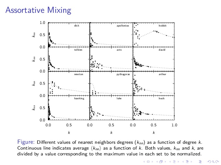
centralities. Assortativity plots, which previous literature claims
to separate fictional from real social networks, were also
studied. We found no relevant differences among genres for the books
studied when applying these network measures and we provide an
explanation why the previous assortativity result is not correct.

Transcript

1. . . . . . . . . . . . . . . . . . . . . . . . . . . . . . . . . . . . . . . . . Character Networks and Book Genre Classification Adriano J. Holanda, Osame Kinouchi FFCLRP–USP May 29, 2019
2. . . . . . . . . . . . . . . . . . . . . . . . . . . . . . . . . . . . . . . . . Research Team Adriano J. Holanda Departamento de Computação e Matemática – FFCLRP Universidade de São Paulo (USP) aholanda@usp.br Mariane Matias Departamento de Física – FFCLRP/USP Sueli M.S.P. Ferreira Departamento de Educação, Informação e Comunicação – FFCLRP/USP Gisele M.L. Benevides Prefeitura do Campus da USP de Ribeirão Preto Osame Kinouchi Departamento de Física - FFCLRP/USP okinouchi@gmail.com
3. . . . . . . . . . . . . . . . . . . . . . . . . . . . . . . . . . . . . . . . . Introduction
4. . . . . . . . . . . . . . . . . . . . . . . . . . . . . . . . . . . . . . . . . Introduction ▶ Recently social networks gathered from literary texts has received some attention. ▶ Most of the analyses characterized the networks of pure fictional texts with different indexes. ▶ Tests of automatic social network extraction algorithms. ▶ Claim that some measures (degree, clustering coefficient, assortativity) can distinguish character networks from real social networks [1, 2].
5. . . . . . . . . . . . . . . . . . . . . . . . . . . . . . . . . . . . . . . . . Introduction ▶ Recently social networks gathered from literary texts has received some attention. ▶ Most of the analyses characterized the networks of pure fictional texts with different indexes. ▶ Tests of automatic social network extraction algorithms. ▶ Claim that some measures (degree, clustering coefficient, assortativity) can distinguish character networks from real social networks [1, 2].
6. . . . . . . . . . . . . . . . . . . . . . . . . . . . . . . . . . . . . . . . . Introduction ▶ Recently social networks gathered from literary texts has received some attention. ▶ Most of the analyses characterized the networks of pure fictional texts with different indexes. ▶ Tests of automatic social network extraction algorithms. ▶ Claim that some measures (degree, clustering coefficient, assortativity) can distinguish character networks from real social networks [1, 2].
7. . . . . . . . . . . . . . . . . . . . . . . . . . . . . . . . . . . . . . . . . Introduction ▶ Recently social networks gathered from literary texts has received some attention. ▶ Most of the analyses characterized the networks of pure fictional texts with different indexes. ▶ Tests of automatic social network extraction algorithms. ▶ Claim that some measures (degree, clustering coefficient, assortativity) can distinguish character networks from real social networks [1, 2].
8. . . . . . . . . . . . . . . . . . . . . . . . . . . . . . . . . . . . . . . . . Objective and Some Applications Social character networks comparison among biographical, legendary and fictional texts, in search for marks of genre differentiation. Some applications: ▶ Automation of book categorization; ▶ Recommender systems.
9. . . . . . . . . . . . . . . . . . . . . . . . . . . . . . . . . . . . . . . . . Objective and Some Applications Social character networks comparison among biographical, legendary and fictional texts, in search for marks of genre differentiation. Some applications: ▶ Automation of book categorization; ▶ Recommender systems.
10. . . . . . . . . . . . . . . . . . . . . . . . . . . . . . . . . . . . . . . . . Methods
11. . . . . . . . . . . . . . . . . . . . . . . . . . . . . . . . . . . . . . . . . Data Set genre author title label Biographical James Gleick Isaac Newton newton Anthony Peake A Life of Philip K. Dick tick Humphrey Carpenter Tolkien: a Biography tolkien Jane Hawking Travelling to Infinity: The True Story Behind The Theory of Ev- erything hawking Legendary Luke Gospel luke Acts of the Apostles acts Philostratus Life of Apollonius of Tyana apollonius Iamblicus Life of Pytaghoras pytaghoras Fiction Charles Dickens David Copperfield david 1 Mark Twain Huckleberry Finn huck1 J. R. R. Tolkien The Hobbit hobbit Bernard Cornwell The Winter King: a novel of Arthur arthur 1Stanford GraphBase, Donald Knuth.
12. . . . . . . . . . . . . . . . . . . . . . . . . . . . . . . . . . . . . . . . . Network Creation Apollonius therefore ranged the Ephesians around him and said: “Pick up as many stones as you can and hurl them at this enemy of the gods.” . . . a demon . . . who resembled in form and look a Molossian dog . . . (Apollonius of Tyana, Book IV, Chapter 10) AP Apollonius of Tyana ... DE demon (4.10) who transform in form and look of a Molossian dog ... EP Ephesians ... ... 4.10:AP,DE,EP;... ... AP DE EP w = 1 weight w = 2 encounters w = 1 distance d = 1/w = 1/2
13. . . . . . . . . . . . . . . . . . . . . . . . . . . . . . . . . . . . . . . . . Network Creation Apollonius therefore ranged the Ephesians around him and said: “Pick up as many stones as you can and hurl them at this enemy of the gods.” . . . a demon . . . who resembled in form and look a Molossian dog . . . (Apollonius of Tyana, Book IV, Chapter 10) AP Apollonius of Tyana ... DE demon (4.10) who transform in form and look of a Molossian dog ... EP Ephesians ... ... 4.10:AP,DE,EP;... ... AP DE EP w = 1 weight w = 2 encounters w = 1 distance d = 1/w = 1/2
14. . . . . . . . . . . . . . . . . . . . . . . . . . . . . . . . . . . . . . . . . Density × Clustering Coefficient Density ρ(G) = 2m n(n − 1) , (1) m – number of edges |E|; n – number of vertices |V|. Clustering Coefficient c(G) = 1 n ∑ v∈G 2 l (v) deg(v) (deg(v) − 1) , (2) deg(v) – number of neighbors of vertex v (degree); l (v) – number of edges between the deg(v) neighbors of vertex v.
15. . . . . . . . . . . . . . . . . . . . . . . . . . . . . . . . . . . . . . . . . Density × Clustering Coefficient Density ρ(G) = 2m n(n − 1) , (1) m – number of edges |E|; n – number of vertices |V|. Clustering Coefficient c(G) = 1 n ∑ v∈G 2 l (v) deg(v) (deg(v) − 1) , (2) deg(v) – number of neighbors of vertex v (degree); l (v) – number of edges between the deg(v) neighbors of vertex v.
16. . . . . . . . . . . . . . . . . . . . . . . . . . . . . . . . . . . . . . . . . Centrality Indices Degree centrality D(v) = deg(v)/(n − 1); (3) Betweenness B(v) = ∑ u̸=v̸=w σuw(v) σuw ; (4) σuw(v) – the number of shortest paths from u to w that pass through v; σuw – number of shortest paths from u to v.
17. . . . . . . . . . . . . . . . . . . . . . . . . . . . . . . . . . . . . . . . . Centrality Indices Degree centrality D(v) = deg(v)/(n − 1); (3) Betweenness B(v) = ∑ u̸=v̸=w σuw(v) σuw ; (4) σuw(v) – the number of shortest paths from u to w that pass through v; σuw – number of shortest paths from u to v.
18. . . . . . . . . . . . . . . . . . . . . . . . . . . . . . . . . . . . . . . . . Centrality Indices Closeness C(v) = ∑ w∈V 1 d(u, w) (5) d(u, v) – shortest distance between v and w normalization – Cmax(v) = 1. Lobby index maximum index i of v such that v has at least i neighbors with degree greater than or equal to i.
19. . . . . . . . . . . . . . . . . . . . . . . . . . . . . . . . . . . . . . . . . Centrality Indices Closeness C(v) = ∑ w∈V 1 d(u, w) (5) d(u, v) – shortest distance between v and w normalization – Cmax(v) = 1. Lobby index maximum index i of v such that v has at least i neighbors with degree greater than or equal to i.
20. . . . . . . . . . . . . . . . . . . . . . . . . . . . . . . . . . . . . . . . . Centrality Indices Closeness C(v) = ∑ w∈V 1 d(u, w) (5) d(u, v) – shortest distance between v and w normalization – Cmax(v) = 1. Lobby index maximum index i of v such that v has at least i neighbors with degree greater than or equal to i. vertices degree index 9 1 7 2 6 3 4 4 3 5
21. . . . . . . . . . . . . . . . . . . . . . . . . . . . . . . . . . . . . . . . . Centrality Indices Closeness C(v) = ∑ w∈V 1 d(u, w) (5) d(u, v) – shortest distance between v and w normalization – Cmax(v) = 1. Lobby index maximum index i of v such that v has at least i neighbors with degree greater than or equal to i. vertices degree index 9 1 7 2 6 3 4 ≤ 4 ← L 3 5
22. . . . . . . . . . . . . . . . . . . . . . . . . . . . . . . . . . . . . . . . . Centrality Indices Closeness C(v) = ∑ w∈V 1 d(u, w) (5) d(u, v) – shortest distance between v and w normalization – Cmax(v) = 1. Lobby index maximum index i of v such that v has at least i neighbors with degree greater than or equal to i. vertices degree index 20 1 7 2 4 3 3 4 2 5
23. . . . . . . . . . . . . . . . . . . . . . . . . . . . . . . . . . . . . . . . . Centrality Indices Closeness C(v) = ∑ w∈V 1 d(u, w) (5) d(u, v) – shortest distance between v and w normalization – Cmax(v) = 1. Lobby index maximum index i of v such that v has at least i neighbors with degree greater than or equal to i. vertices degree index 20 1 7 2 4 ≤ 3 ← L 3 4 2 5
24. . . . . . . . . . . . . . . . . . . . . . . . . . . . . . . . . . . . . . . . . Centralities Correlation ▶ Linear correlation ⇒ Lobby × {degree, closeness, betweenness} ▶ Why not all combinations? ▶ Focus on Lobby → least studied index.
25. . . . . . . . . . . . . . . . . . . . . . . . . . . . . . . . . . . . . . . . . Centralities Correlation ▶ Linear correlation ⇒ Lobby × {degree, closeness, betweenness} ▶ Why not all combinations? ▶ Focus on Lobby → least studied index.
26. . . . . . . . . . . . . . . . . . . . . . . . . . . . . . . . . . . . . . . . . Assortativity Mixing Average degree k of neighbors of v ⟨knn(v)⟩ = ∑ u,v ∈V∧{u,v}∈E deg(u) {|U| : U ⊆ V ∧ ∀u ∈ U → {u, v} ∈ E} (6) assortative mixing - positive slope of the curve is, disassortative mixing - negative slope.
27. . . . . . . . . . . . . . . . . . . . . . . . . . . . . . . . . . . . . . . . . Power Law of Degree Distribution Empirical degree distribution using the method developed by Clauset et al. [3] to fit the curves to a power law distribution.
28. . . . . . . . . . . . . . . . . . . . . . . . . . . . . . . . . . . . . . . . . Hapax Legomena Number of v (characters) whose frequency of appearance is equal to 1. HL = {|U| : U ⊆ V ∧ ∀u ∈ U → freq(u) = 1}/n. (7)
29. . . . . . . . . . . . . . . . . . . . . . . . . . . . . . . . . . . . . . . . . Results
30. . . . . . . . . . . . . . . . . . . . . . . . . . . . . . . . . . . . . . . . . Global measures Table: Basic parameters of data set, average degree ⟨d⟩, and global network measures density ρ and clustering coefficient c. genre book n m ⟨d⟩ Biography Dick 115 189 3.29±7.27 Tolkien 94 219 4.66±9.04 Newton 33 44 2.67±3.29 Hawking 249 446 3.58±11.51 Legendary Apollonius 95 138 2.91±7.37 Acts 76 160 4.21±5.14 Pythagoras 41 31 1.51±2.18 Luke 76 203 5.34±8.10 Fiction Hobbit 41 160 7.80±7.43 David 87 406 9.33±10.49 Arthur 77 141 3.66±5.98 Huck 74 301 8.14±7.34
31. . . . . . . . . . . . . . . . . . . . . . . . . . . . . . . . . . . . . . . . . Degree Distribution 10−2 10−1 100 10−2 10−1 100 10−2 10−1 10−2 10−1 10−2 10−1 10−2 10−1 10−2 10−1 100 101 10−2 10−1 100 101 100 101 100 101 100 101 102 100 101 102 Pr(X ≥ x) dick α = 2.71 p > 0.05∗ ˆ xmin Pr(X ≥ x) dick α = 2.71 p > 0.05∗ ˆ xmin apollonius α = 2.43 p > 0.05∗ ˆ xmin apollonius α = 2.43 p > 0.05∗ ˆ xmin hobbit α = 1.50 p < 0.05 ˆ xmin = 1 hobbit α = 1.50 p < 0.05 ˆ xmin = 1 Pr(X ≥ x) tolkien α = 2.66 p > 0.05∗ ˆ xmin Pr(X ≥ x) tolkien α = 2.66 p > 0.05∗ ˆ xmin acts α = 3.41 p > 0.05∗ ˆ xmin acts α = 3.41 p > 0.05∗ ˆ xmin david α = 3.49 p > 0.05∗ ˆ xmin david α = 3.49 p > 0.05∗ ˆ xmin Pr(X ≥ x) newton α = 2.95 p > 0.05∗ ˆ xmin Pr(X ≥ x) newton α = 2.95 p > 0.05∗ ˆ xmin pythagoras α = 2.93 p > 0.05∗ ˆ xmin = 1 pythagoras α = 2.93 p > 0.05∗ ˆ xmin = 1 arthur α = 2.30 p > 0.05∗ ˆ xmin arthur α = 2.30 p > 0.05∗ ˆ xmin Pr(X ≥ x) x hawking α = 2.54 p > 0.05∗ ˆ xmin Pr(X ≥ x) x hawking α = 2.54 p > 0.05∗ ˆ xmin x luke α = 2.26 p < 0.05 ˆ xmin x luke α = 2.26 p < 0.05 ˆ xmin x huck α = 3.50 p < 0.05 ˆ xmin x huck α = 3.50 p < 0.05 ˆ xmin Figure: Cumulative degree distribution function Pr(X ≥ x) of character networks for all books’ data set. The dashed lines represent the maximum likelihood power-law fits that start at ˆ xmin and follow a power-law distribution f(x) = x−α, α > 1, x ≥ ˆ xmin > 0. The p-values marked with ∗ are statistically significant (p > 0.05).
32. . . . . . . . . . . . . . . . . . . . . . . . . . . . . . . . . . . . . . . . . Density × Clustering Coefficient 0 0.2 0.4 0.6 0.8 1 0 0.05 0.1 0.15 0.2 f(x) = 4x − 0.04 r = 0.93, p = 9.75e − 06 clustering coefficient density dick (B) apollonius (L) hobbit (F) tolkien (B) acts (L) david (F) newton (B) pythagoras (L) arthur (F) hawking (B) luke (L) huck (F) Figure: Correlation between density and clustering coefficient. (The books’ genres are written between parenthesis after their labels: B means biography, F is for fiction and L for legendary.)
33. . . . . . . . . . . . . . . . . . . . . . . . . . . . . . . . . . . . . . . . . Degree × Lobby 0.0 0.25 0.5 0.0 0.25 0.5 0.0 0.25 0.0 0.25 0.0 0.25 0.0 0.25 0.0 0.25 0.0 0.5 0.0 0.25 0.0 0.5 0.0 0.5 0.0 0.5 0.0 0.5 1.0 0.0 0.5 1.0 Lobby dick r = 0.52 p ≪ 0.05∗ Lobby dick r = 0.52 p ≪ 0.05∗ apollonius r = 0.48 p ≪ 0.05∗ apollonius r = 0.48 p ≪ 0.05∗ hobbit r = 0.95 p ≪ 0.05∗ hobbit r = 0.95 p ≪ 0.05∗ Lobby tolkien r = 0.62 p ≪ 0.05∗ Lobby tolkien r = 0.62 p ≪ 0.05∗ acts r = 0.65 p ≪ 0.05∗ acts r = 0.65 p ≪ 0.05∗ david r = 0.77 p ≪ 0.05∗ david r = 0.77 p ≪ 0.05∗ Lobby newton r = 0.58 p ≪ 0.05∗ Lobby newton r = 0.58 p ≪ 0.05∗ pythagoras r = 0.11 p > 0.05 pythagoras r = 0.11 p > 0.05 arthur r = 0.76 p ≪ 0.05∗ arthur r = 0.76 p ≪ 0.05∗ Lobby D hawking r = 0.50 p ≪ 0.05∗ Lobby D hawking r = 0.50 p ≪ 0.05∗ D luke r = 0.71 p ≪ 0.05∗ D luke r = 0.71 p ≪ 0.05∗ D huck r = 0.68 p ≪ 0.05∗ D huck r = 0.68 p ≪ 0.05∗ Figure: Dispersion plots for Lobby vs degree centrality with Pearson correlation r at the top. The p-values marked with ∗ are statistically significant (p < 0.05). (Some plots, like Pythagoras, show few points because they have the same (L, D) coordinates.)
34. . . . . . . . . . . . . . . . . . . . . . . . . . . . . . . . . . . . . . . . . Betweenness × Lobby 0.0 0.25 0.5 0.0 0.25 0.5 0.0 0.25 0.0 0.25 0.0 0.25 0.0 0.25 0.0 0.25 0.0 0.5 0.0 0.25 0.0 0.5 0.0 0.5 0.0 0.5 0.0 0.5 1.0 0.0 0.5 1.0 Lobby dick r = 0.38 p ≪ 0.05∗ Lobby dick r = 0.38 p ≪ 0.05∗ apollonius r = 0.40 p ≪ 0.05∗ apollonius r = 0.40 p ≪ 0.05∗ hobbit r = 0.31 p > 0.05 hobbit r = 0.31 p > 0.05 Lobby tolkien r = 0.43 p ≪ 0.05∗ Lobby tolkien r = 0.43 p ≪ 0.05∗ acts r = 0.35 p ≪ 0.05∗ acts r = 0.35 p ≪ 0.05∗ david r = 0.53 p ≪ 0.05∗ david r = 0.53 p ≪ 0.05∗ Lobby newton r = 0.40 p ≪ 0.05∗ Lobby newton r = 0.40 p ≪ 0.05∗ pythagoras r = −0.04 p > 0.05 pythagoras r = −0.04 p > 0.05 arthur r = 0.52 p ≪ 0.05∗ arthur r = 0.52 p ≪ 0.05∗ Lobby betweenness hawking r = 0.42 p ≪ 0.05∗ Lobby betweenness hawking r = 0.42 p ≪ 0.05∗ betweenness luke r = 0.30 p ≪ 0.05∗ betweenness luke r = 0.30 p ≪ 0.05∗ betweenness huck r = 0.24 p ≪ 0.05∗ betweenness huck r = 0.24 p ≪ 0.05∗ Figure: Correlation plots for Lobby betweenness centrality with Pearson correlation r at the top. The p-values marked with ∗ are statistically significant (p < 0.05).
35. . . . . . . . . . . . . . . . . . . . . . . . . . . . . . . . . . . . . . . . . Closeness × Lobby 0.0 0.25 0.5 0.0 0.25 0.5 0.0 0.25 0.0 0.25 0.0 0.25 0.0 0.25 0.0 0.25 0.0 0.5 0.0 0.25 0.0 0.5 0.0 0.5 0.0 0.5 0.0 0.5 1.0 0.0 0.5 1.0 Lobby dick r = −0.14 p > 0.05 Lobby dick r = −0.14 p > 0.05 apollonius r = −0.27 p ≪ 0.05∗ apollonius r = −0.27 p ≪ 0.05∗ hobbit r = 0.89 p ≪ 0.05∗ hobbit r = 0.89 p ≪ 0.05∗ Lobby tolkien r = 0.16 p > 0.05 Lobby tolkien r = 0.16 p > 0.05 acts r = −0.07 p > 0.05 acts r = −0.07 p > 0.05 david r = 0.62 p ≪ 0.05∗ david r = 0.62 p ≪ 0.05∗ Lobby newton r = 0.39 p ≪ 0.05∗ Lobby newton r = 0.39 p ≪ 0.05∗ pythagoras r = 0.11 p > 0.05 pythagoras r = 0.11 p > 0.05 arthur r = 0.24 p ≪ 0.05∗ arthur r = 0.24 p ≪ 0.05∗ Lobby closeness hawking r = 0.00 p > 0.05 Lobby closeness hawking r = 0.00 p > 0.05 closeness luke r = 0.01 p > 0.05 closeness luke r = 0.01 p > 0.05 closeness huck r = −0.19 p > 0.05 closeness huck r = −0.19 p > 0.05 Figure: Correlation plots for Lobby vs closeness centrality with Pearson correlation r at the top. The p-values marked with ∗ are statistically significant (p < 0.05).
36. . . . . . . . . . . . . . . . . . . . . . . . . . . . . . . . . . . . . . . . . Assortative Mixing 0.0 0.5 1.0 dick apollonius hobbit 0.0 0.5 tolkien acts david 0.0 0.5 newton pythagoras arthur 0.0 0.5 0.0 0.5 hawking 0.0 0.5 luke 0.0 0.5 1.0 huck knn knn knn knn k k k Figure: Different values of nearest neighbors degrees (knn) as a function of degree k. Continuous line indicates average ⟨knn⟩ as a function of k. Both values, knn and k, are divided by a value corresponding to the maximum value in each set to be normalized.
37. . . . . . . . . . . . . . . . . . . . . . . . . . . . . . . . . . . . . . . . . Hapax Legomena Table: Hapax legomena normalized by the number of characters n. Table: Biography book HL Tolkien 0.46 Dick 0.39 Hawking 0.31 Newton 0.30 Table: Legendary book HL Pythagoras 0.83 Luke 0.67 Acts 0.67 Apollonius 0.65 Table: Fiction book HL Huck 0.43 Arthur 0.40 David 0.30 Hobbit 0.17
38. . . . . . . . . . . . . . . . . . . . . . . . . . . . . . . . . . . . . . . . . Discussion
39. . . . . . . . . . . . . . . . . . . . . . . . . . . . . . . . . . . . . . . . . Categorization is Hard ▶ Alberich et al.: differences between the average degree and clustering coefficients of the Marvel Universe (MU) network and social networks (movie actors, scientific collaboration) [1].
40. . . . . . . . . . . . . . . . . . . . . . . . . . . . . . . . . . . . . . . . . Categorization is Hard ▶ Gleiser: MU is very different from real social networks because it is disassortative [2].
41. . . . . . . . . . . . . . . . . . . . . . . . . . . . . . . . . . . . . . . . . Categorization is Hard ▶ Alberich et al.: differences between the average degree and clustering coefficients of the Marvel Universe (MU) network and social networks [1]. (biographical-like) ▶ Gleiser: MU is very different from real social networks because it is disassortative [2]. (biographical-like) ▶ Low average degree, low clustering coefficient and disassortative behavior also found in biographical (real-life) character networks.
42. . . . . . . . . . . . . . . . . . . . . . . . . . . . . . . . . . . . . . . . . ▶ A legendary or biographical text ≈ few characters with high degree and some edges with high weight. ▶ The same arrangement normally doesn’t occur with fictional texts. Apollonius of Tyana (L) book (n = 93, m = 138) wmax = 35 (27% of the encounters) ⇒ Apollonius (k = 72) and Damis (k = 12); Huckleberry Finn (F) (n = 74, m = 301) wmax = 28 (5.2% of the encounters) ⇒ Huckleberry (k = 53) and Jim (k = 16); Stephen Hawking (B) (n = 248, m = 444) wmax = 108 (24.2%) ⇒ Hawking (k = 99) and Jane (k = 152); David Copperfield (F) (n = 87, m = 406) wmax = 54 (13.3%) ⇒ David (k = 82) and Betsey (k = 31).
43. . . . . . . . . . . . . . . . . . . . . . . . . . . . . . . . . . . . . . . . . ▶ A legendary or biographical text ≈ few characters with high degree and some edges with high weight. ▶ The same arrangement normally doesn’t occur with fictional texts. Apollonius of Tyana (L) book (n = 93, m = 138) wmax = 35 (27% of the encounters) ⇒ Apollonius (k = 72) and Damis (k = 12); Huckleberry Finn (F) (n = 74, m = 301) wmax = 28 (5.2% of the encounters) ⇒ Huckleberry (k = 53) and Jim (k = 16); Stephen Hawking (B) (n = 248, m = 444) wmax = 108 (24.2%) ⇒ Hawking (k = 99) and Jane (k = 152); David Copperfield (F) (n = 87, m = 406) wmax = 54 (13.3%) ⇒ David (k = 82) and Betsey (k = 31).
44. . . . . . . . . . . . . . . . . . . . . . . . . . . . . . . . . . . . . . . . . ▶ A legendary or biographical text ≈ few characters with high degree and some edges with high weight. ▶ The same arrangement normally doesn’t occur with fictional texts. Apollonius of Tyana (L) book (n = 93, m = 138) wmax = 35 (27% of the encounters) ⇒ Apollonius (k = 72) and Damis (k = 12); Huckleberry Finn (F) (n = 74, m = 301) wmax = 28 (5.2% of the encounters) ⇒ Huckleberry (k = 53) and Jim (k = 16); Stephen Hawking (B) (n = 248, m = 444) wmax = 108 (24.2%) ⇒ Hawking (k = 99) and Jane (k = 152); David Copperfield (F) (n = 87, m = 406) wmax = 54 (13.3%) ⇒ David (k = 82) and Betsey (k = 31).
45. . . . . . . . . . . . . . . . . . . . . . . . . . . . . . . . . . . . . . . . . Categorization with Centrality Indices ▶ Ronqui and Travieso: analysis of correlations between centrality indexes to characterize and distinguish between natural and artificial networks [4].
46. . . . . . . . . . . . . . . . . . . . . . . . . . . . . . . . . . . . . . . . . Categorization with Centrality Indices ▶ Ronqui and Travieso: analysis of correlations between centrality indexes to characterize and distinguish between natural and artificial networks [4]. ▶ Lobby × {degree, closeness, betweenness} are very similar between genres.
47. . . . . . . . . . . . . . . . . . . . . . . . . . . . . . . . . . . . . . . . . Degree Distribution Power Law-like f(x) = x−α ▶ Exponent range α: 2.3 − 3.49; ▶ Fictional: 2.3 − 3.49, ▶ Legendary: 2.43 − 3.41, ▶ Biographical: 2.66 − 2.95. ▶ Same exponent range of biographical: ▶ Yeast protein interactions (biological): 2.89; ▶ E. Coli outdegree (biological): 2.9; ▶ Citation network: 2.9. Alberich et al. → α = 3.12 for Marvel Universe (F) [1].
48. . . . . . . . . . . . . . . . . . . . . . . . . . . . . . . . . . . . . . . . . Degree Distribution Power Law-like f(x) = x−α ▶ Exponent range α: 2.3 − 3.49; ▶ Fictional: 2.3 − 3.49, ▶ Legendary: 2.43 − 3.41, ▶ Biographical: 2.66 − 2.95. ▶ Same exponent range of biographical: ▶ Yeast protein interactions (biological): 2.89; ▶ E. Coli outdegree (biological): 2.9; ▶ Citation network: 2.9. Alberich et al. → α = 3.12 for Marvel Universe (F) [1].
49. . . . . . . . . . . . . . . . . . . . . . . . . . . . . . . . . . . . . . . . . Conclusions ▶ Automatic classification of books in genres is a hard task; ▶ Indices used in our study helped increase the knowledge about the character network structure; ▶ Our study can be used as a starting point or benchmark to other studies in the field.
50. . . . . . . . . . . . . . . . . . . . . . . . . . . . . . . . . . . . . . . . . Conclusions ▶ Automatic classification of books in genres is a hard task; ▶ Indices used in our study helped increase the knowledge about the character network structure; ▶ Our study can be used as a starting point or benchmark to other studies in the field.
51. . . . . . . . . . . . . . . . . . . . . . . . . . . . . . . . . . . . . . . . . Conclusions ▶ Automatic classification of books in genres is a hard task; ▶ Indices used in our study helped increase the knowledge about the character network structure; ▶ Our study can be used as a starting point or benchmark to other studies in the field.
52. . . . . . . . . . . . . . . . . . . . . . . . . . . . . . . . . . . . . . . . . Challenges ahead ▶ Automation of graph creation; ▶ Study of network dynamics.
53. . . . . . . . . . . . . . . . . . . . . . . . . . . . . . . . . . . . . . . . . Challenges ahead ▶ Automation of graph creation; ▶ Study of network dynamics.
54. . . . . . . . . . . . . . . . . . . . . . . . . . . . . . . . . . . . . . . . . Acknowledgments ▶ FAPESP, grant 2013/07699-0; ▶ CNPq; ▶ Núcleo de Apoio á Pesquisa CNAIPS-USP; ▶ PUB–USP; ▶ Reviewers and editors.
55. . . . . . . . . . . . . . . . . . . . . . . . . . . . . . . . . . . . . . . . . References R. Alberich, J. Miro-Julia, and F. Rosselló, “Marvel universe looks almost like a real social network,” arXiv preprint cond-mat/0202174, 2002. P. M. Gleiser, “How to become a superhero,” J. Stat. Mech. Theor. Exp, vol. 2007, no. 09, p. P09020, 2007. A. Clauset, C. R. Shalizi, and M. E. J. Newman, “Power-law distributions in empirical data,” SIAM Rev., vol. 51, no. 4, pp. 661–703, 2009. J. R. F. Ronqui and G. Travieso, “Analyzing complex networks through correlations in centrality measurements,” J. Stat. Mech. Theor. Exp, vol. 2015, no. 5, p. P05030, 2015.
56. . . . . . . . . . . . . . . . . . . . . . . . . . . . . . . . . . . . . . . . . Reproducibility ▶ Source code, data set, manuscript: https://ajholanda.github.io/charnet/