CellIQ: Real-Time Cellular Network Analytics at Scale

Presented at NSDI 2015

Transcript

1. CellIQ: Real-Time Cellular Network
   Analytics at Scale
   Anand Iyer#, Li Erran Li+, Ion Stoica#
   #UC Berkeley +Bell Labs
   

   View Slide

2. Cellular Networks have been
   seeing exponential growth
   and become part of our lives
   

   View Slide

3. Image courtesy: Alcatel-Lucent
   

   View Slide

4. What is needed to solve these issues?
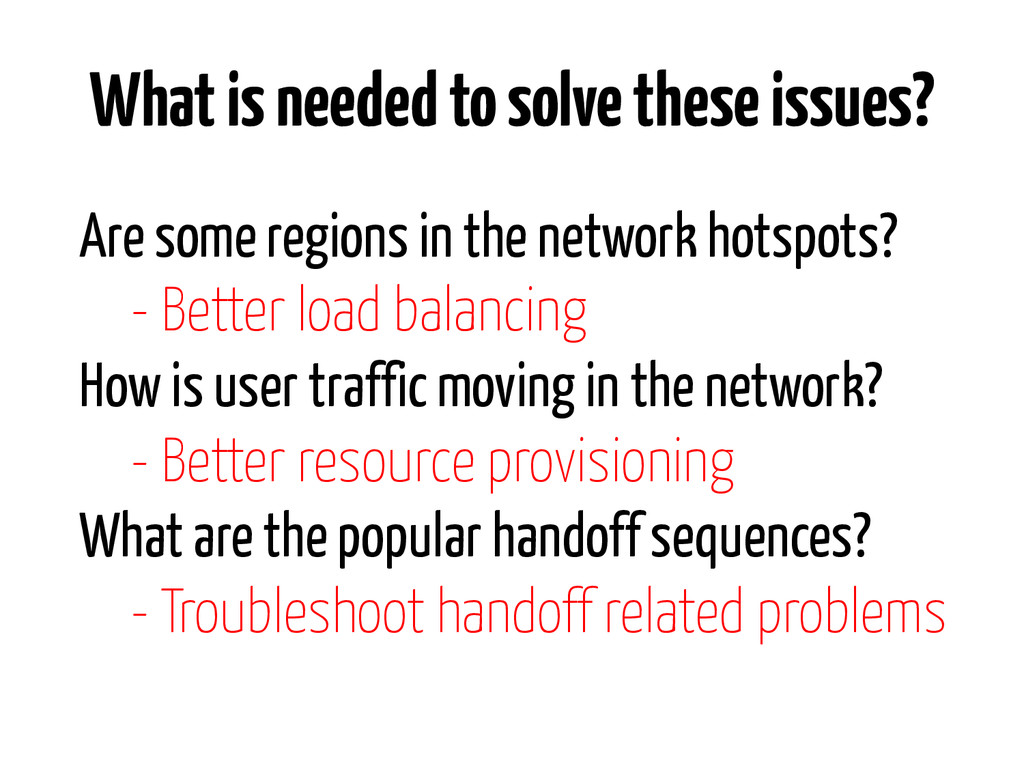
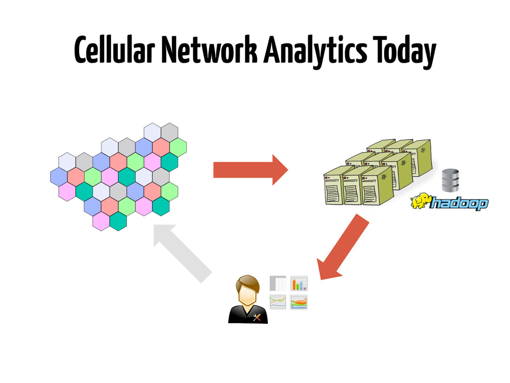
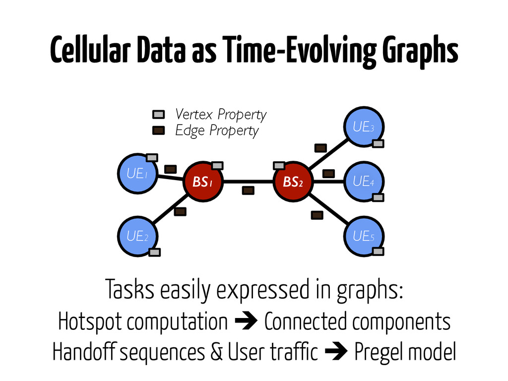
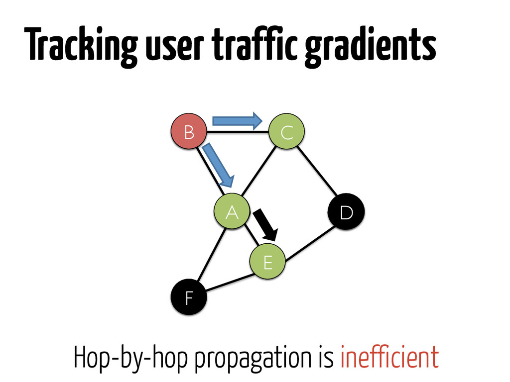
   Are some regions in the network hotspots?
   - Better load balancing
   How is user traffic moving in the network?
   - Better resource provisioning
   What are the popular handoff sequences?
   - Troubleshoot handoff related problems
   

   View Slide

5. Cellular Network Analytics Today
   

   View Slide

6. Cellular Network Analytics Today
   

   View Slide

7. Cellular Network Analytics Today
   

   View Slide

8. Problem
   Existing cellular network
   analytic systems do not
   support advanced analytic
   tasks in an efficient manner.
   

   View Slide

9. High Velocity Data
   Continuous Monitoring
   Advanced Tasks
   Timely Spatio-Temporal Analysis
   Challenges
   

   View Slide

10. CellIQ is a cellular network analytics
    system that supports rich analysis
    tasks efficiently by leveraging
    domain-specific optimizations
    

    View Slide

11. Cellular Data as Time-Evolving Graphs
    Tasks easily expressed in graphs:
    Hotspot computation è Connected components
    Handoff sequences & User traffic è Pregel model
    Edge Property
    Vertex Property
    BS1
    UE2
    UE1 BS2
    UE3
    UE4
    UE5
    

    View Slide

12. Why Not Use a Graph Parallel Framework?
    ��
    ��
    ���
    ���
    ���
    ���
    ���
    ���
    ���
    �������� ���������� ������ �����
    �����������������������
    ������������
    Fails to produce results!
    Domain specific optimizations key for efficient analysis
    

    View Slide

13. CellIQ Implementation
    *Gonzales. et.al. “GraphX: Graph Processing in a Distributed Dataflow Framework”, OSDI 2014
    Implemented as a layer on GraphX*
    Incorporates several domain specific optimizations
    GraphX
    Spark
    Pregel API
    PageRank Connected Comp. K-core
    Triangle
    Count
    LDA SVD++
    CellIQ
    

    View Slide

14. Computational Model
    BS1
    UE2
    UE1
    BS2
    UE3
    UE4
    UE5
    

    View Slide

15. Computational Model
    BS1
    UE2
    UE1
    BS2
    UE3
    UE4
    UE5
    BS1
    UE2
    UE1
    BS2
    UE3
    UE4
    UE5
    

    View Slide

16. Computational Model
    BS1
    UE2
    UE1
    BS2
    UE3
    UE4
    UE5
    BS1
    UE2
    UE1
    BS2
    UE3
    UE4
    UE5
    BS1
    UE2
    UE1 BS2
    UE3
    UE4
    UE5
    

    View Slide

17. Computational Model: GStreams
    BS1
    UE2
    UE1
    BS2
    UE3
    UE4
    UE5
    BS1
    UE2
    UE1
    BS2
    UE3
    UE4
    UE5
    BS1
    UE2
    UE1 BS2
    UE3
    UE4
    UE5
    Domain specific graph partitioning
    Spatial operations
    Window operations
    

    View Slide

18. Computational Model: GStreams
    BS1
    UE2
    UE1
    BS2
    UE3
    UE4
    UE5
    BS1
    UE2
    UE1
    BS2
    UE3
    UE4
    UE5
    BS1
    UE2
    UE1 BS2
    UE3
    UE4
    UE5
    Domain specific graph partitioning
    Spatial operations
    Window operations
    

    View Slide

19. Graph computation frameworks rely on partitioning
    to minimize communication & balance computation
     
    B C
    A D
    F
    E
    A D
    D
    B C
    D
    E
    A
    A
    F Machine 1 Machine 2
    A
    B
    C
    D
    E
    F
    Graph Partitioning
    

    View Slide

20. Partition geographically close-by entities
     
    Machine 3 Machine 4
    3
    B C
    B C
    D
    E
    A
    F
    Machine 1 Machine 2
    CellIQ Graph Partitioning
    G H
    2D 1D
    ?
    

    View Slide

21. 3
    Machine 3 Machine 4
    B C
    B C
    D
    E
    A
    F
    Machine 1 Machine 2
    A
    B
    C
    D
    E
    F
    Graph Partitioning
    G H
    G
    H
    Random (hashed) partitioning
    

    View Slide

22. 3
    Machine 3 Machine 4
    B C
    B C
    D
    E
    A
    F
    Machine 1 Machine 2
    A
    B
    C
    D
    E
    F
    Graph Partitioning
    G H
    G
    H
    Random (hashed) partitioning
    results in poor spatial locality
    

    View Slide

23. Machine 3 Machine 4
    B C
    B C
    D
    E
    A
    F
    Machine 1 Machine 2
    CellIQ Graph Partitioning
    G H
    Uses Hilbert space-filling curves
    

    View Slide

24. Machine 3 Machine 4
    0 3
    2
    1
    B C
    B C
    D
    E
    A
    F
    Machine 1 Machine 2
    CellIQ Graph Partitioning
    G H
    Uses Hilbert space-filling curves
    Use curve’s distance as the 1-dimensional key
    

    View Slide

25. Machine 3 Machine 4
    0 3
    2
    1
    B C
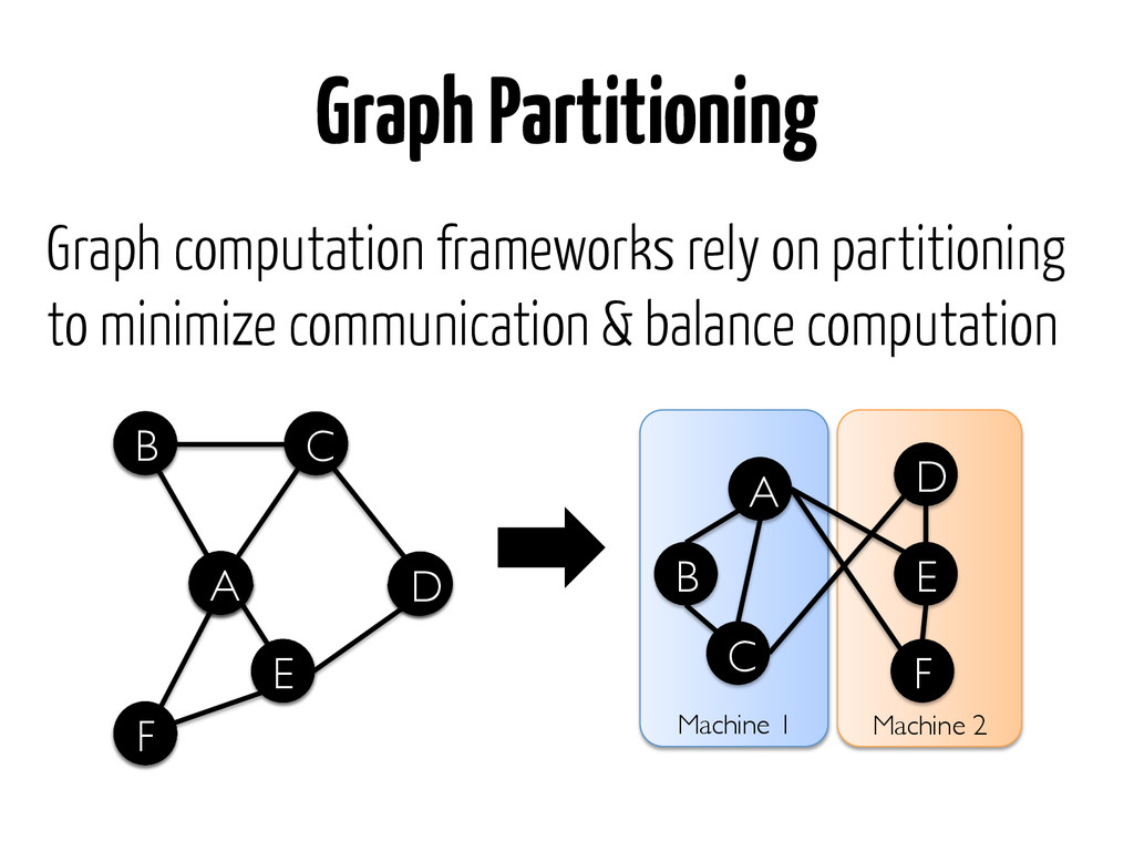
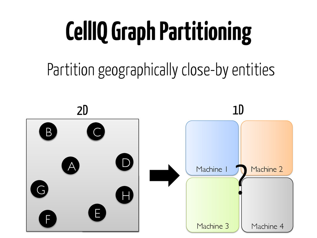
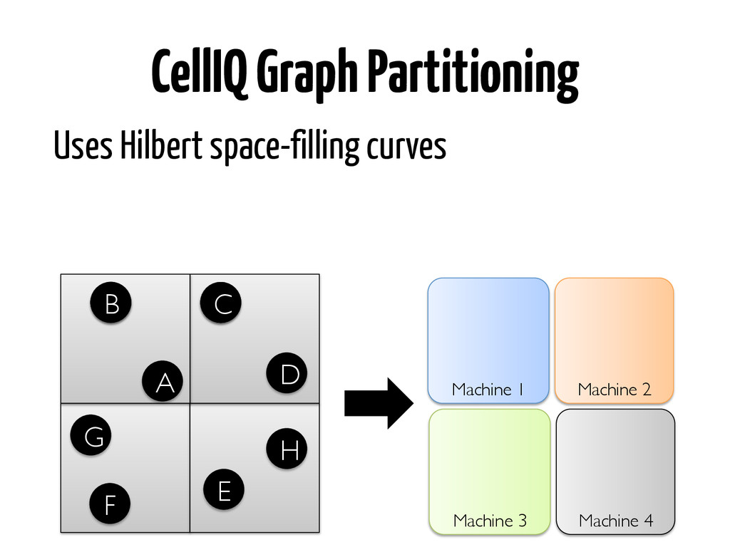
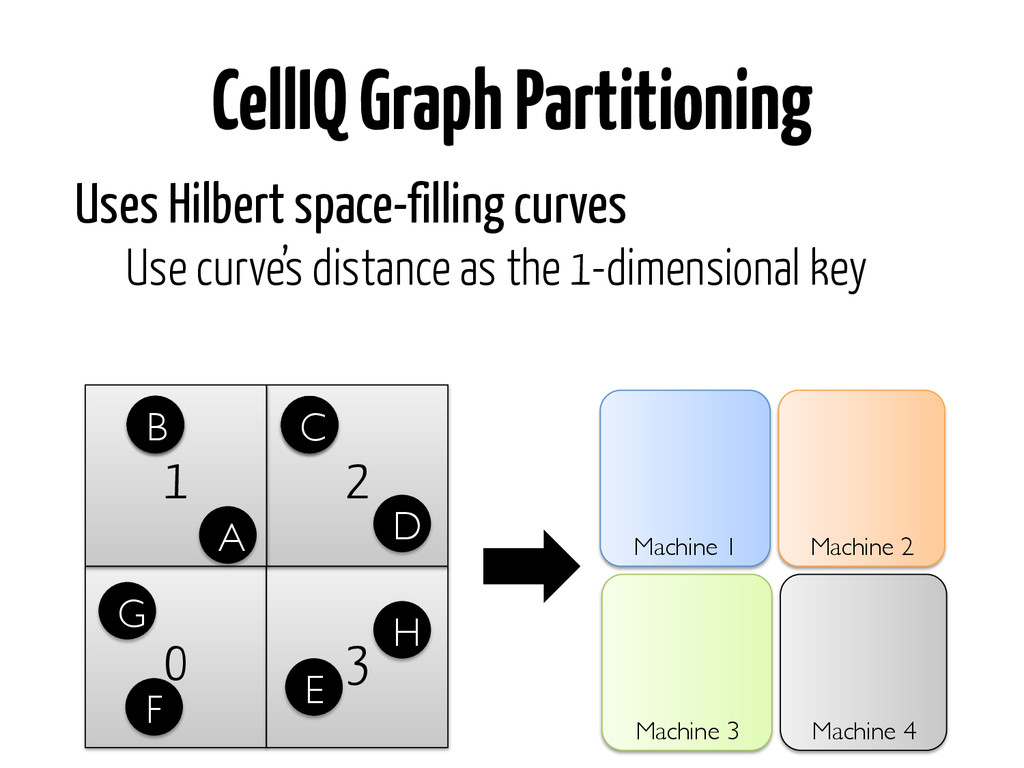
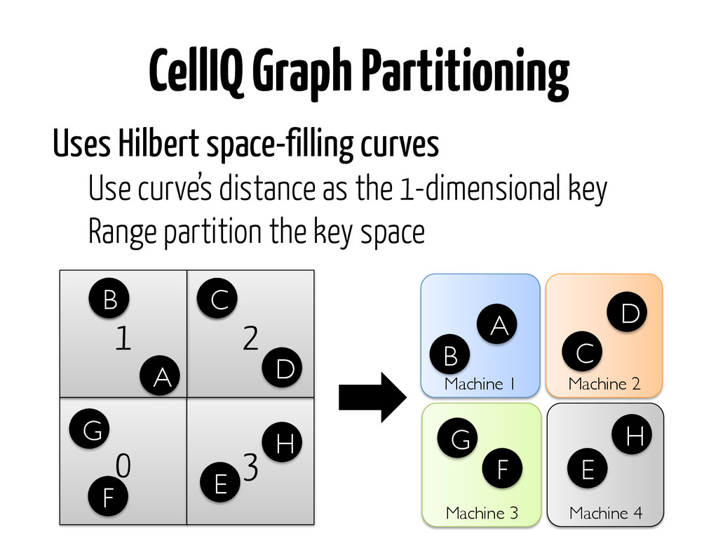
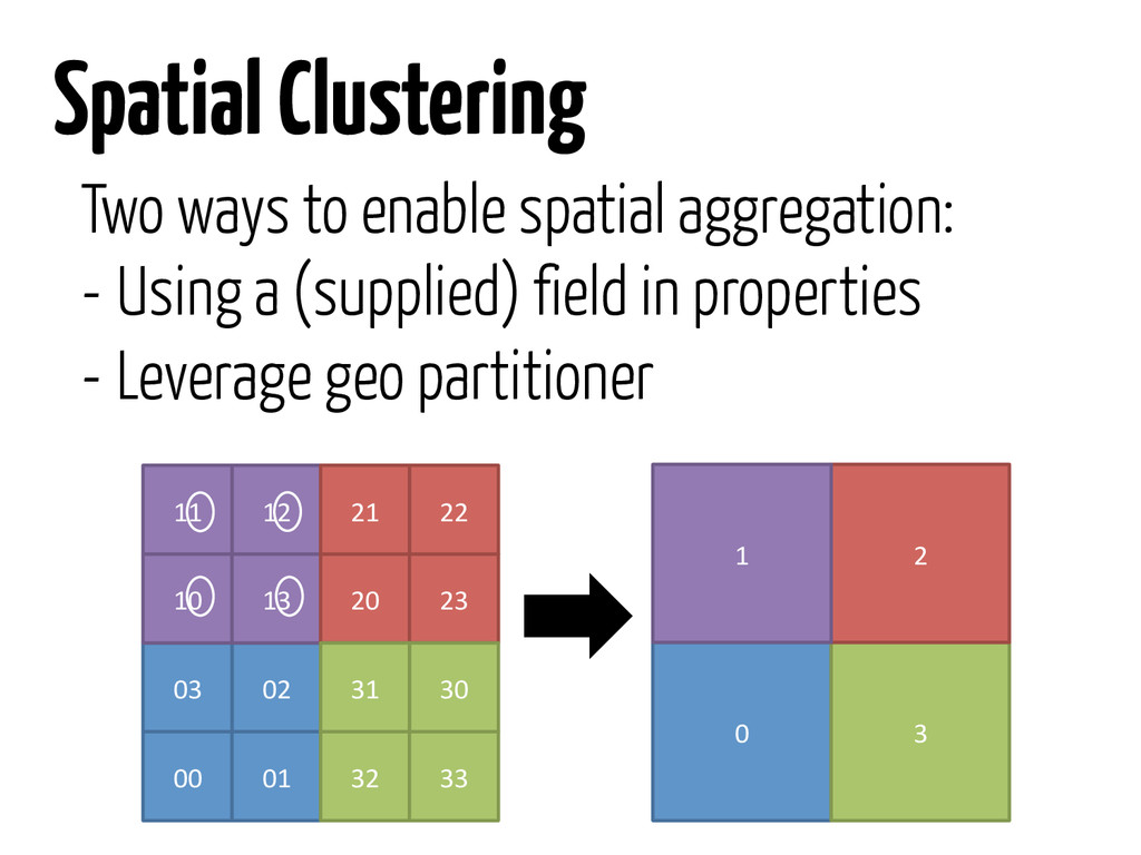
    B C
    D
    E
    A
    F
    Machine 1 Machine 2
    A
    B C
    D
    E
    F
    CellIQ Graph Partitioning
    G H G H
    Uses Hilbert space-filling curves
    Use curve’s distance as the 1-dimensional key
    Range partition the key space
    

    View Slide

26. 0 1
    2
    3
    4 7
    6
    5
    8 11
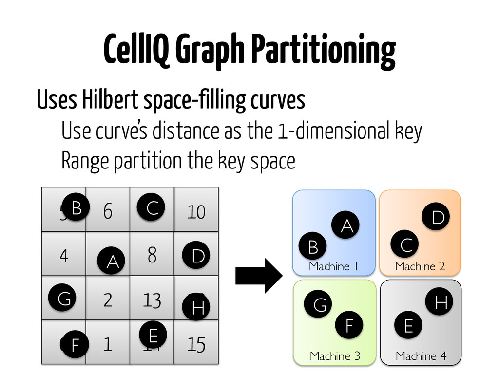
    10
    9
    14 15
    12
    13
    Machine 3 Machine 4
    B C
    B C
    D
    E
    A
    F
    Machine 1 Machine 2
    A
    B C
    D
    E
    F
    CellIQ Graph Partitioning
    G H G H
    Uses Hilbert space-filling curves
    Use curve’s distance as the 1-dimensional key
    Range partition the key space
    

    View Slide

27. Computational Model: GStreams
    BS1
    UE2
    UE1
    BS2
    UE3
    UE4
    UE5
    BS1
    UE2
    UE1
    BS2
    UE3
    UE4
    UE5
    BS1
    UE2
    UE1 BS2
    UE3
    UE4
    UE5
    Domain specific graph partitioning
    Spatial operations
    Window operations
    

    View Slide

28. GeoGraph API
    class  GeoGraph[V,  E]  {  
       //  Broadcast  a  message  to  all    
       //  vertices  within  a  radius  
       def  sendMsg(radius)  
         
       //  Create  a  spatially  aggregated    
       //  graph  by  combining  vertices      
       //  and  edges    
       def  spatialAG(reduceV:  (V,  V)  =>  V,  
                                   reduceE:  (E,  E)  =>  E)  
    }  
    

    View Slide

29. Tracking user traffic gradients
    Goal: Detect and track
    direction of movement of
    user groups
    

    View Slide

30. 3
    B C
    A D
    F
    E
    A D
    D
    B C
    D
    E
    A
    A
    F
    Tracking user traffic gradients
    Base Station
    

    View Slide

31. 3
    B C
    A D
    F
    E
    A D
    D
    B C
    D
    E
    A
    A
    F
    Tracking user traffic gradients
    

    View Slide

32. B C
    A D
    F
    E
    A D
    D
    B C
    D
    E
    A
    A
    F
    Hop-by-hop propagation
    Tracking user traffic gradients
    

    View Slide

33. B C
    A D
    F
    E
    A D
    D
    B C
    D
    E
    A
    A
    F
    Hop-by-hop propagation is inefficient
    Tracking user traffic gradients
    

    View Slide

34. Tracking user traffic gradients
    B C
    A D
    F
    E
    A D
    D
    B C
    D
    E
    A
    A
    F
    Instead, CellIQ enables radius based broadcast
    

    View Slide

35. Part. 2
    Part. 1
    Vertex Table
    (RDD)
    B C
    A D
    F
    E
    A D
    Routing Table in GraphX enables Multicast
    D
    B C
    D
    E
    A
    A
    F
    Machine 1 Machine 2
    Edge Table
    (RDD)
    A B
    A C
    C D
    B C
    A E
    A F
    E F
    E D
    B
    C
    D
    E
    A
    F
    Routing
    Table
    (RDD)
    B
    C
    D
    E
    A
    F
    1  
    2  
    1   2  
    1   2  
    1  
    2  
    Slide courtesy: Joey Gonzales
    

    View Slide

36. Routing
    Table
    (RDD)
    B
    C
    D
    E
    A
    F
    1  
    2  
    1   2  
    1   2  
    1  
    2  
    Part. 2
    Part. 1
    Vertex Table
    (RDD)
    B C
    A D
    F
    E
    A D
    D
    B C
    D
    E
    A
    A
    F
    Machine 1 Machine 2
    Edge Table
    (RDD)
    A B
    A C
    C D
    B C
    A E
    A F
    E F
    E D
    B
    C
    D
    E
    A
    F
    Slide courtesy: Joey Gonzales
    Can compute destination partitions easily due to the use
    of geo-partitioner
    

    View Slide

37. GeoGraph API
    class  GeoGraph[V,  E]  {  
       //  Broadcast  a  message  to  all    
       //  vertices  within  a  radius  
       def  sendMsg(radius)  
         
       //  Create  a  spatially  aggregated    
       //  graph  by  combining  vertices      
       //  and  edges    
       def  spatialAG(reduceV:  (V,  V)  =>  V,  
                                   reduceE:  (E,  E)  =>  E)  
    }  
    

    View Slide

38. B C
    A D
    F
    E
    A D
    D
    B C
    D
    E
    A
    A
    F
    Spatial Clustering
    F E D
    D
    B’
    F
    Goal: Combine spatially
    close-by vertices
    

    View Slide

39. Spatial Clustering
    Two ways to enable spatial aggregation:
    - Using a (supplied) field in properties
    - Leverage geo partitioner
    00   01  
    02  
    03  
    10   13  
    12  
    11  
    20   23  
    22  
    21  
    32   33  
    30  
    31  
    

    View Slide

40. Spatial Clustering
    Two ways to enable spatial aggregation:
    - Using a (supplied) field in properties
    - Leverage geo partitioner
    00   01  
    02  
    03  
    10   13  
    12  
    11  
    20   23  
    22  
    21  
    32   33  
    30  
    31  
    0   3  
    2  
    1  
    

    View Slide

41. Computational Model: GStreams
    BS1
    UE2
    UE1
    BS2
    UE3
    UE4
    UE5
    BS1
    UE2
    UE1
    BS2
    UE3
    UE4
    UE5
    BS1
    UE2
    UE1 BS2
    UE3
    UE4
    UE5
    Domain specific graph partitioning
    Spatial operations
    Window operations
    

    View Slide

42. Tracking Persistent Hotspots
    Goal: Detect and track
    groups of base stations
    with high traffic volume
    Equivalent to finding connected components
    

    View Slide

43. Tracking Persistent Hotspots
    BS1
    BS2 BS3
    t1 t2 t3
    W
    Combining graphs at the end of the window
    results in many join operations (inefficient)
    BS1
    BS2
    BS1
    BS2
    

    View Slide

44. Tracking Persistent Hotspots
    BS1
    BS2 BS3
    t1 t2 t3
    W
    BS1
    BS2
    BS1
    BS2
    BS1
    BS2 BS3
    1 1
    1
    BS1
    BS2 BS3
    2 1
    1
    BS1
    BS2 BS3
    3 1
    1
    Apply incremental updates to a cumulative graph
    

    View Slide

45. Tracking Persistent Hotspots
    BS1
    BS2 BS3
    t1 t2 t3
    BS1
    BS2
    BS1
    BS2
    BS1
    BS2 BS3
    1
    1
    1
    Apply differential updates to a cumulative graph
    BS1
    BS3
    t4
    BS1
    BS2 BS3
    1
    2
    1
    BS1
    BS2 BS3
    1
    3
    1
    BS1
    BS2 BS3
    1
    2
    0
    

    View Slide

46. GStream API
    class  GStream[V,  E]  {  
     
       def  graphReduceByWindow(  
           reduceFunc(Graph[V,  E],  Graph[V,  E],    
                                 fv:  (V,  V)  =>  V,    
                                 fe:  (E,  E)  =>  E):  Graph[V,  E],    
           invReduceFunc(Graph[V,  E],  Graph[V,  E],    
                                 fv:  (V,  V)  =>  V,    
                                 fe:  (E,  E)  =>  E):  Graph[V,  E],    
           windowDuration,  slideDuration)  
    }  
    

    View Slide

47. graphReduceByWindow    
    •  Implemented using Spark’s cogroupedRDD  
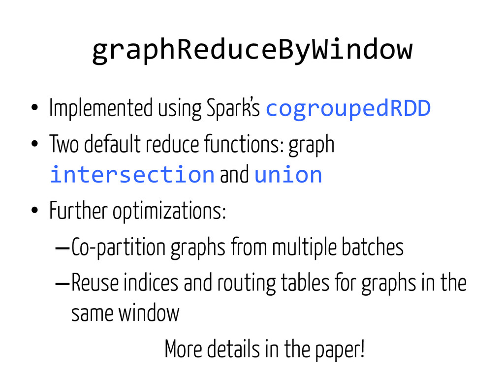
    •  Two default reduce functions: graph
    intersection and union
    •  Further optimizations:
    – Co-partition graphs from multiple batches
    – Reuse indices and routing tables for graphs in the
    same window
    More details in the paper!
    

    View Slide

48. How does CellIQ perform?
    

    View Slide

49. Evaluation Setup
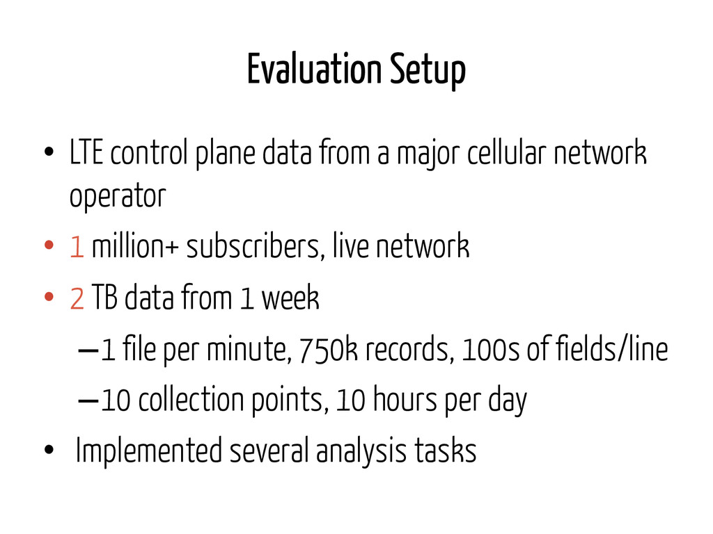
    •  LTE control plane data from a major cellular network
    operator
    •  1 million+ subscribers, live network
    •  2 TB data from 1 week
    – 1 file per minute, 750k records, 100s of fields/line
    – 10 collection points, 10 hours per day
    •  Implemented several analysis tasks
    

    View Slide

50. Benefits of Geo-partitioning
    ��
    ��
    ���
    ���
    ���
    ���
    ���
    ���
    ���
    �������� ���������� ������ �����
    �����������������������
    ������������
    �������������������� ����������������
    

    View Slide

51. Benefits of Geo-partitioning
    ��
    ��
    ���
    ���
    ���
    ���
    ���
    ���
    ���
    �������� ���������� ������ �����
    �����������������������
    ������������
    �������������������� ����������������
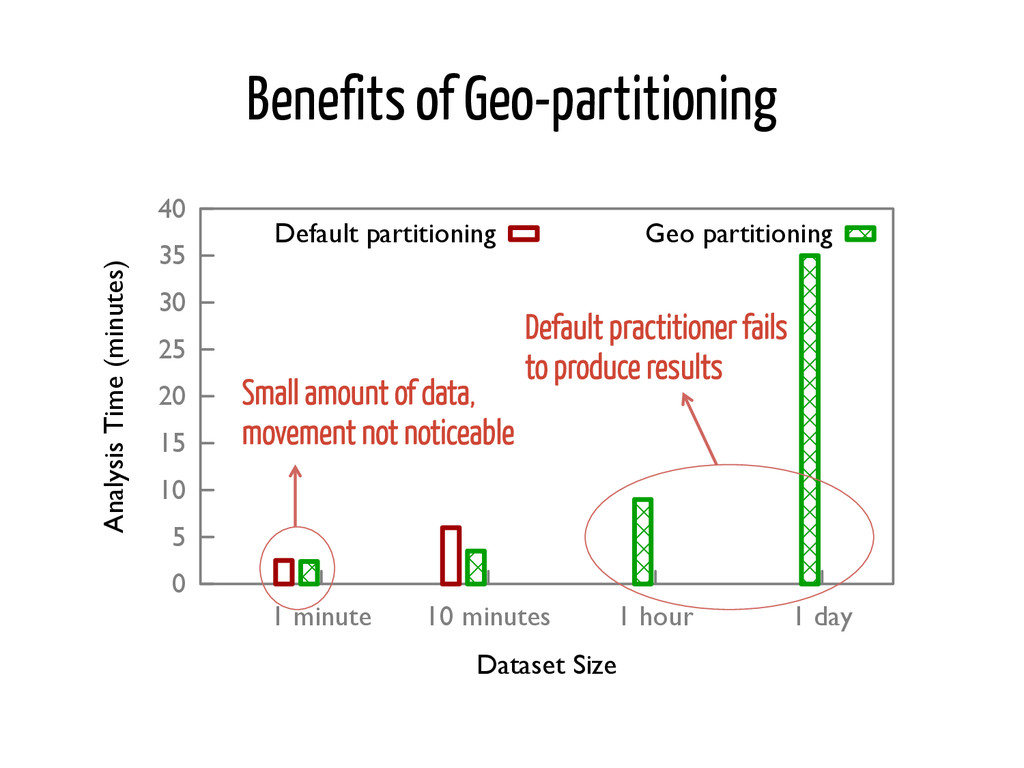
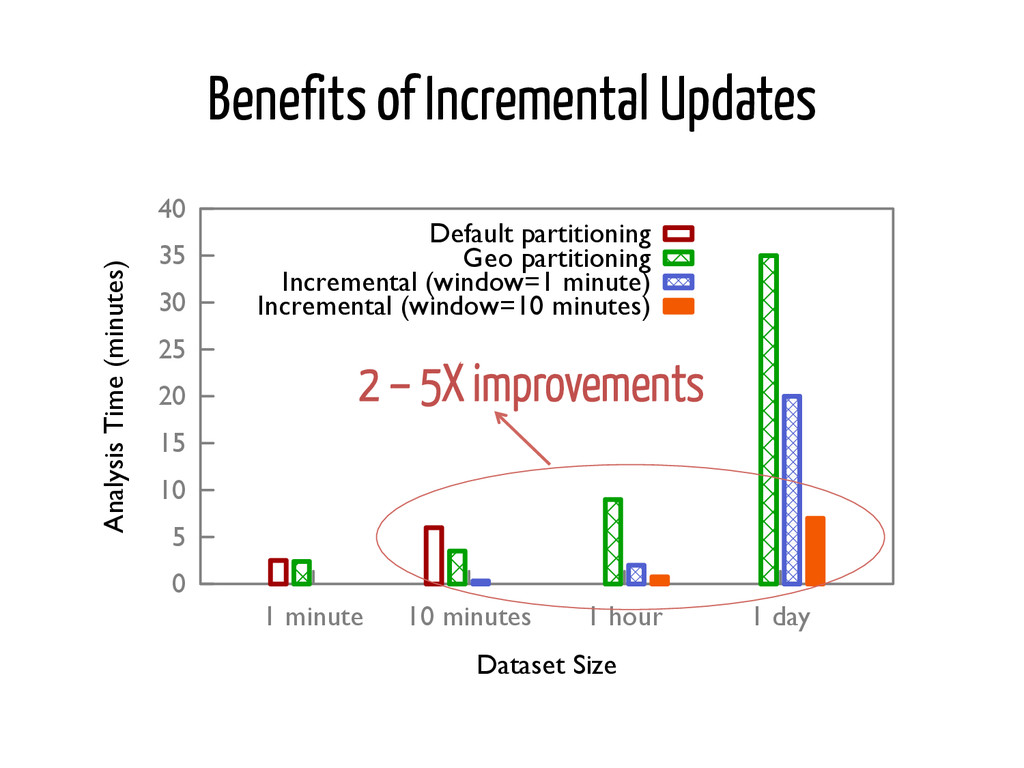
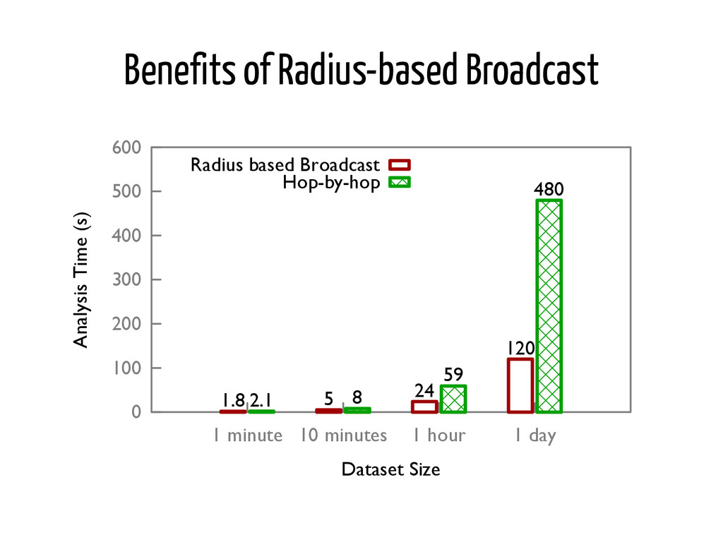
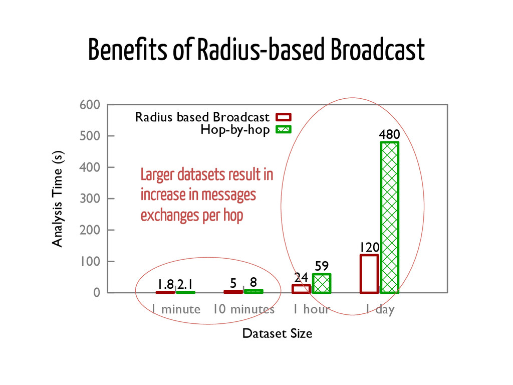
    Small amount of data,
    movement not noticeable
    Default practitioner fails
    to produce results
    

    View Slide

52. Benefits of Incremental Updates
    ��
    ��
    ���
    ���
    ���
    ���
    ���
    ���
    ���
    �������� ���������� ������ �����
    �����������������������
    ������������
    ��������������������
    ����������������
    �����������������������������
    �������������������������������
    

    View Slide

53. Benefits of Incremental Updates
    ��
    ��
    ���
    ���
    ���
    ���
    ���
    ���
    ���
    �������� ���������� ������ �����
    �����������������������
    ������������
    ��������������������
    ����������������
    �����������������������������
    �������������������������������
    2 – 5X improvements
    

    View Slide

54. Benefits of Incremental Updates
    ��
    ��
    ���
    ���
    ���
    ���
    ���
    ���
    ���
    �������� ���������� ������ �����
    �����������������������
    ������������
    ��������������������
    ����������������
    �����������������������������
    �������������������������������
    window size affects
    performance
    

    View Slide

55. Benefits of Differential Updates
    ��
    ��
    ��
    ��
    ��
    ���
    �� �� �� �� �� ��� ���
    �����������������
    ����������������
    ��������
    ������
    

    View Slide

56. Benefits of Differential Updates
    ��
    ��
    ��
    ��
    ��
    ���
    �� �� �� �� �� ��� ���
    �����������������
    ����������������
    ��������
    ������
    Larger windows see
    bigger benefits
    Graceful degradation in
    performance
    

    View Slide

57. Benefits of Radius-based Broadcast
    ��
    ����
    ����
    ����
    ����
    ����
    ����
    �������� ���������� ������ �����
    �����������������
    ������������
    ����������������������
    ��� � ��
    ���
    ����������
    ��� �
    ��
    ���
    

    View Slide

58. Benefits of Radius-based Broadcast
    ��
    ����
    ����
    ����
    ����
    ����
    ����
    �������� ���������� ������ �����
    �����������������
    ������������
    ����������������������
    ��� � ��
    ���
    ����������
    ��� �
    ��
    ���
    Larger datasets result in
    increase in messages
    exchanges per hop
    

    View Slide

59. CellIQ is a cellular network analytics
    system that uses domain-specific
    optimizations to achieve 2x to 5x
    improvements
    

    View Slide

60. CellIQ is a cellular network analytics
    system that uses domain-specific
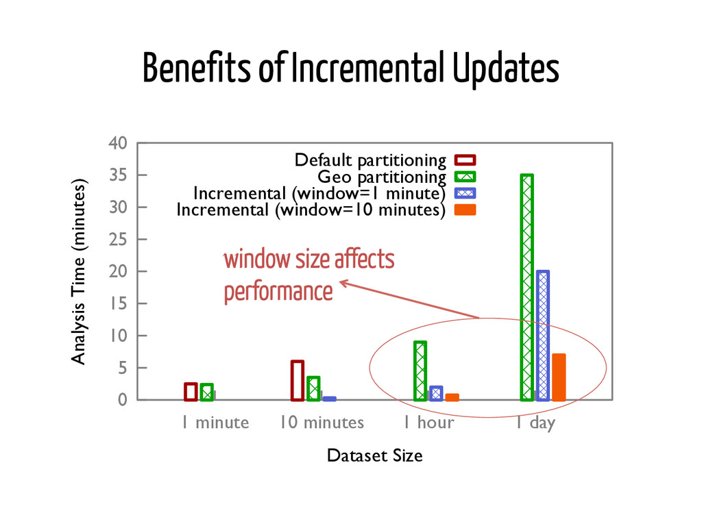
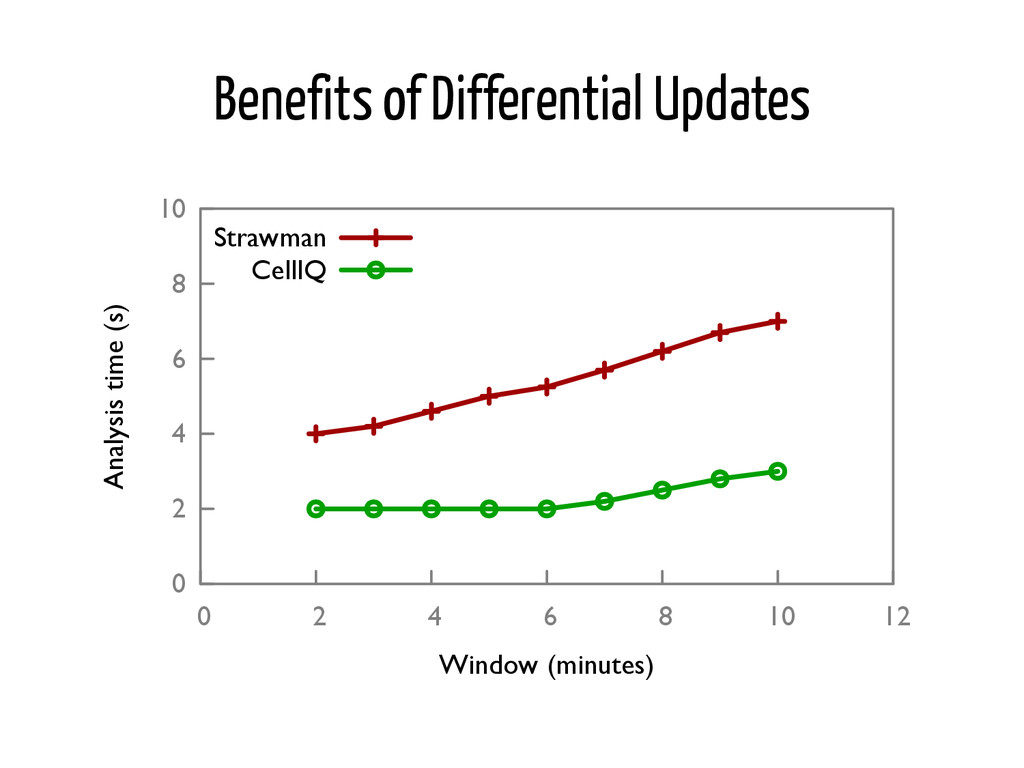
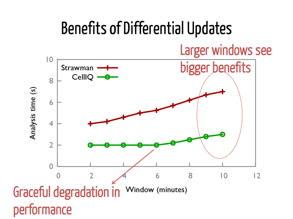
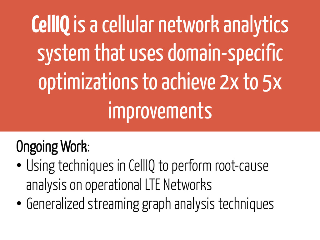
    optimizations to achieve 2x to 5x
    improvements
    Ongoing Work:
    • Using techniques in CellIQ to perform root-cause
    analysis on operational LTE Networks
    • Generalized streaming graph analysis techniques
    

    View Slide