A randomized pairwise likelihood method for complex statistical inferences

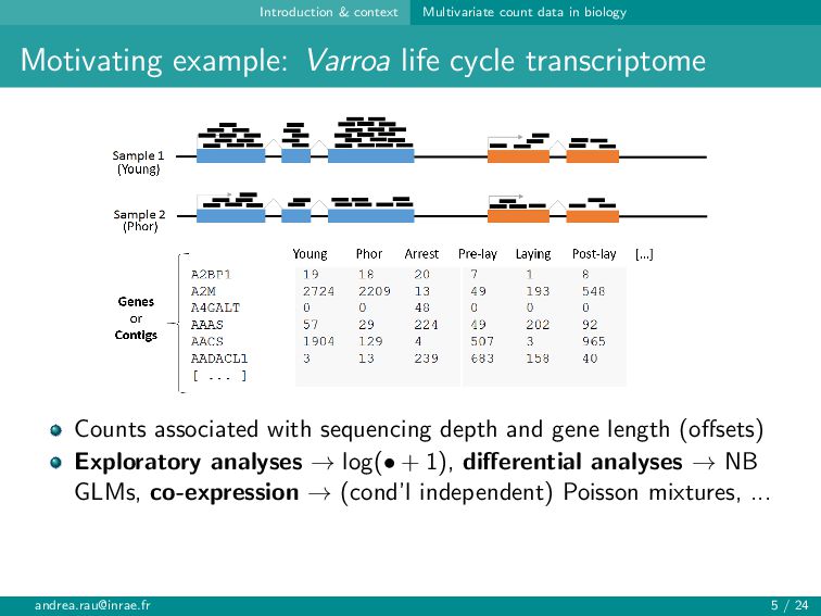
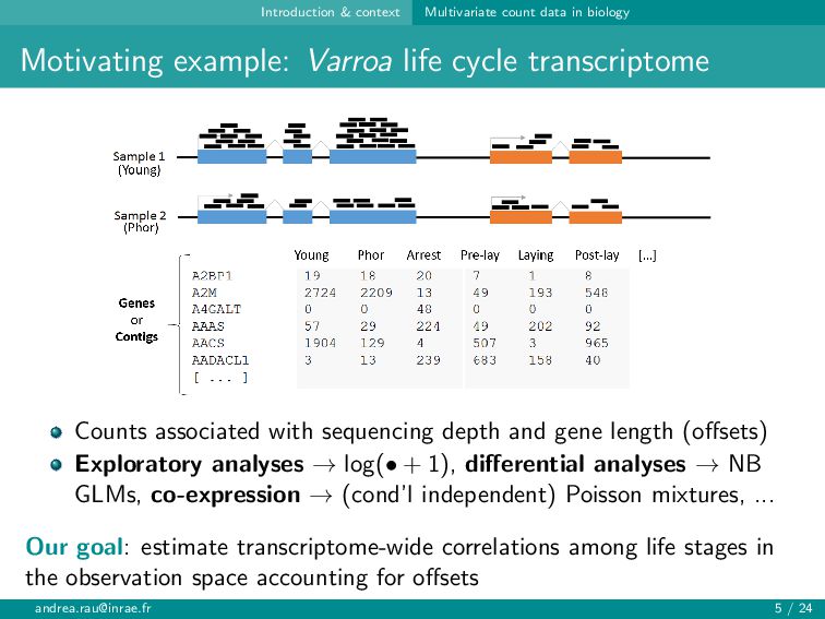
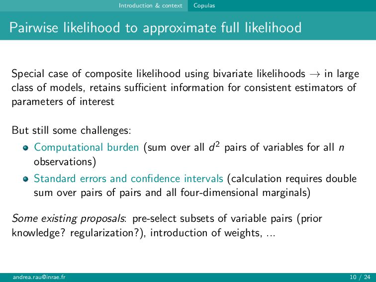
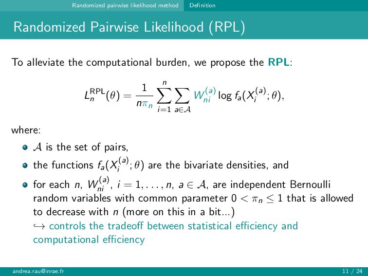
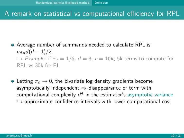
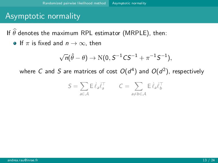
Pairwise likelihood methods are commonly used for inference in parametric statistical models in cases where the full likelihood is too complex to be used, such as multivariate count data. Although pairwise likelihood methods represent a useful solution to perform inference for intractable likelihoods, several computational challenges remain, particularly in higher dimensions. To alleviate these issues, we consider a randomized pairwise likelihood approach, where only summands randomly sampled across observations and pairs are used for the estimation. In addition to the usual tradeoff between statistical and computational efficiency, we show that, under a condition on the sampling parameter, this two-way random sampling mechanism allows for the construction of less computationally expensive confidence intervals. The proposed approach, which is implemented in the rpl R package, is illustrated in tandem with copula-based models for multivariate count data in simulations and on a set of transcriptomic data.

(Joint work with Gildas Mazo and Dimitris Karlis)

Transcript

1. A randomized pairwise likelihood method for complex statistical inferences Gildas Mazo, Dimitris Karlis, and Andrea Rau February 7, 2022 S´ eminaire Parisien de Statistique @ IHP, Paris andrea.rau@inrae.fr 1 / 24
2. Outline 1 Introduction & context 2 Randomized pairwise likelihood method 3 Numerical illustrations 4 RNA-seq data analysis 5 rpl R package 6 Discussion & conclusion andrea.rau@inrae.fr 2 / 24
3. Introduction & context Multivariate count data in biology Multivariate counts in biology Multivariate count data are routinely collected by biologists: Animal traits relevant to production (number of eggs laid), reproduction (litter size), immunity (number of monocytes), ... Plant phenotypes relevant to physiology (number of leaves), development (number of flowering plants per parcel), yield (number of seeds per plant), ... Microbial ecology (counts of bacterial species in a given ecosystem) High-throughput sequencing data: counts of sequenced reads associated with a given biological entity andrea.rau@inrae.fr 3 / 24
4. Introduction & context Multivariate count data in biology Motivating example: Varroa life cycle transcriptome Mondet et al. (2018) Varroa destructor is a parasitic mite that is a major threat to the western honeybee Impact on bees well-studied, but less is known about its functional biology during adult life cycle → collect transcriptome catalog Image adapted from Mondet et al. (2018) and https://flickr.com/photos/54563451@N08/48697155713 andrea.rau@inrae.fr 4 / 24
5. Introduction & context Multivariate count data in biology Motivating example: Varroa life cycle transcriptome Counts associated with sequencing depth and gene length (offsets) Exploratory analyses → log(• + 1), differential analyses → NB GLMs, co-expression → (cond’l independent) Poisson mixtures, ... andrea.rau@inrae.fr 5 / 24
6. Introduction & context Multivariate count data in biology Motivating example: Varroa life cycle transcriptome Counts associated with sequencing depth and gene length (offsets) Exploratory analyses → log(• + 1), differential analyses → NB GLMs, co-expression → (cond’l independent) Poisson mixtures, ... Our goal: estimate transcriptome-wide correlations among life stages in the observation space accounting for offsets andrea.rau@inrae.fr 5 / 24
7. Introduction & context Multivariate count data in biology Logs or latent variables for multivariate count data Multivariate Poisson Log-Normal distribution (Aitchison & Ho, 1989) Variational probabilistic Poisson PCA (Chiquet et al. 2018) ... andrea.rau@inrae.fr 6 / 24
8. Introduction & context Copulas What is a copula? A copula, among other things, is a multivariate c.d.f. C whose arguments are in (0, 1). Any multivariate joint distribution can be expressed as a function (copula) of its marginal c.d.f.’s (Sklar’s theorem): F(x1, . . . , xd ) = C(F1(x1), . . . , Fd (xd )), as if we were “adding a dependence structure” on top of sets of independent random variables → Build multivariate models with prescribed marginal distributions Many families of copulas available + easily analyze behavior of system under different (1) correlation structures or (2) marginals andrea.rau@inrae.fr 7 / 24
9. Introduction & context Copulas Modeling multivariate count data with copulas The following choices, as a first approximation, may be reasonable to build a multivariate statistical model for counts: Poisson marginals: Fi (xi ) = Fµi (xi ) A Gaussian copula for the dependence structure, e.g. C(u1, . . . , ud ; ρ) = Φd (Φ−1 1 (u1), . . . , Φ−1 1 (ud ); R(ρ)), where Φd (•; R(ρ)) is the distribution function of a standard d-variate Gaussian distribution with correlation matrix R(ρ) andrea.rau@inrae.fr 8 / 24
10. Introduction & context Copulas The copula inference challenge If it is so easy to build multivariate count models, why is this approach not widespread? One reason is that inference is challenging. The probability density function associated with the above copula model is a sum of 2d terms, given by (v1,...,vd ) sgn(v1, . . . , vd )C(Fµ1 (v1), . . . , Fµd (vd ); ρ), where the sum is over all (v1, . . . , vd ) ∈ {x1 − 1, x1} × . . . × {xd − 1, xd }, and sgn(v1, . . . , vd ) ± 1 (according to the vector’s state) One solution: estimate θ = (µ1, . . . , µd , ρ) with pairwise likelihood methods (Varin et al., 2011) andrea.rau@inrae.fr 9 / 24
11. Introduction & context Copulas Pairwise likelihood to approximate full likelihood Special case of composite likelihood using bivariate likelihoods → in large class of models, retains sufficient information for consistent estimators of parameters of interest But still some challenges: Computational burden (sum over all d2 pairs of variables for all n observations) Standard errors and confidence intervals (calculation requires double sum over pairs of pairs and all four-dimensional marginals) Some existing proposals: pre-select subsets of variable pairs (prior knowledge? regularization?), introduction of weights, ... andrea.rau@inrae.fr 10 / 24
12. Randomized pairwise likelihood method Definition Randomized Pairwise Likelihood (RPL) To alleviate the computational burden, we propose the RPL: LRPL n (θ) = 1 nπn n i=1 a∈A W (a) ni log fa(X(a) i ; θ), where: A is the set of pairs, the functions fa(X(a) i ; θ) are the bivariate densities, and for each n, W (a) ni , i = 1, . . . , n, a ∈ A, are independent Bernoulli random variables with common parameter 0 < πn ≤ 1 that is allowed to decrease with n (more on this in a bit...) → controls the tradeoff between statistical efficiency and computational efficiency andrea.rau@inrae.fr 11 / 24
13. Randomized pairwise likelihood method Definition A remark on statistical vs computational efficiency for RPL Average number of summands needed to calculate RPL is nπnd(d − 1)/2 → Example: if πn = 1/6, d = 3, n = 10k, 5k terms to compute for RPL vs 30k for PL Letting πn → 0, the bivariate log density gradients become asymptotically independent ⇒ disappearance of term with computational complexity d4 in the estimator’s asymptotic variance → approximate confidence intervals with lower computational cost andrea.rau@inrae.fr 12 / 24
14. Randomized pairwise likelihood method Asymptotic normality Asymptotic normality If θ denotes the maximum RPL estimator (MRPLE), then: If π is fixed and n → ∞, then √ n(ˆ θ − θ) → N(0, S−1CS−1 + π−1S−1), where C and S are matrices of cost O(d4) and O(d2), respectively S = a∈A E ˙ a ˙ a C = a=b∈A E ˙ a ˙ b andrea.rau@inrae.fr 13 / 24
15. Randomized pairwise likelihood method Asymptotic normality Asymptotic normality If θ denotes the maximum RPL estimator (MRPLE), then: If π is fixed and n → ∞, then √ n(ˆ θ − θ) → N(0, S−1CS−1 + π−1S−1), where C and S are matrices of cost O(d4) and O(d2), respectively S = a∈A E ˙ a ˙ a C = a=b∈A E ˙ a ˙ b If πn → 0 and some condition that implies nπn → ∞, then √ nπn(ˆ θ − θ) → N(0, S−1), The second result suggests that an approximate standard error of the estimator can be computed with cost O(d2) andrea.rau@inrae.fr 13 / 24
16. Randomized pairwise likelihood method Inflation factor of MRPLE A reasonable inflation of MRPLE asymptotic variance? Consider MRPLE ˆ θMRPL n (π) and V (π) its asymptotic variance Inflation factor from π to π given by: IF(π |π) := V (π ) V (π) = πS−1CS−1 πS−1CS−1 + S−1 + S−1 πS−1CS−1 + S−1 π π When is this inflation factor subhomogeneous, i.e. IF(k−1π|π) < k IF(π|π) = k for all π? andrea.rau@inrae.fr 14 / 24
17. Randomized pairwise likelihood method Inflation factor of MRPLE A reasonable inflation of MRPLE asymptotic variance? Consider MRPLE ˆ θMRPL n (π) and V (π) its asymptotic variance Inflation factor from π to π given by: IF(π |π) := V (π ) V (π) = πS−1CS−1 πS−1CS−1 + S−1 + S−1 πS−1CS−1 + S−1 π π When is this inflation factor subhomogeneous, i.e. IF(k−1π|π) < k IF(π|π) = k for all π? → when S−1CS−1 is nonnegative definite, i.e. when ˙ a, ˙ b, a = b, tend to be positively correlated andrea.rau@inrae.fr 14 / 24
18. Randomized pairwise likelihood method Inflation factor of MRPLE Large enough n, small but not too small πn ...aka large enough nπn So how to choose πn in practice? Under some conditions, choosing πn = n−α, 0 < α < 1/2, makes n(1−α)/2(ˆ θn − θ) go to a Gaussian limit ⇒ πn can decrease almost as fast as 1/ √ n Simulations could help: Identify region in (π, nπ) ∈ (0, a] × [b, ∞) for some constants a and b, where the approximation seems to be “good enough” Choose π within this region and adjust according to acceptable standard errors S−1/(nπ) andrea.rau@inrae.fr 15 / 24
19. Numerical illustrations Effect of π on performance & computational time Description of simulation study: impact of π d = 30, n ∈ {100, 500, 1000} simulated from unit Poisson marginals and Gaussian copula for two different correlation structures × 500 datasets: Factorized (30 distinct copula parameters) Blockwise exchangeable (3 blocks; 6 distinct copula parameters) → Parameter estimates obtained with RPL using π = 0.1, 0.3, 0.5 andrea.rau@inrae.fr 16 / 24
20. Numerical illustrations Effect of π on performance & computational time andrea.rau@inrae.fr 17 / 24
21. Numerical illustrations Effect of π on performance & computational time andrea.rau@inrae.fr 17 / 24
22. Numerical illustrations Effect of π on performance & computational time andrea.rau@inrae.fr 17 / 24
23. Numerical illustrations Coverage of approximate confidence intervals Description of simulation study: approximate CI coverage aka How good is the approximated variance? d = 3, n ∈ {500, 100, 5000} simulated from unit Poisson marginals and Gaussian copula with unstructured correlation × 500 datasets: ρ12 = 0.3, ρ13 = 0.2, ρ23 = 0 “Small π, large nπ” setting → Approximate confidence intervals constructed with RPL using π ∈ [0.01, 0.90] using S−1/(nπ) ⇒ proportion of simulated datasets for which true parameter values were within the 95% confidence intervals andrea.rau@inrae.fr 18 / 24
24. Numerical illustrations Coverage of approximate confidence intervals All coverages exceeding 92% correspond to π ≤ 0.25 and nπ ≥ 125 ⇒ reasonable rule of thumb for choosing π in practice? andrea.rau@inrae.fr 19 / 24
25. RNA-seq data analysis Description Back to the Varroa life cycle RNA-seq data Read counts for n = 22, 372 contigs in d = 10 Varroa life cycle groups from a single colony → transcriptome-wide correlations among life stages Contig lengths ( i ) and TMM-normalized sequencing depth (sj ) considered to be a known terms in offset for marginal Poisson GLMs: log E(Xij ) = log( i sj ) + µj for contig i in life stage j Poisson marginals coupled with an unstructured Gaussian copula → Parameters of interest are θ = (µj , ρj,j ), j = j ∈ {1, . . . , 10} andrea.rau@inrae.fr 20 / 24
26. RNA-seq data analysis RPL results (π = 0.01, nπ = 224) Phor Pre−Lay Non−reproductive Laying Arrest Post−Lay Emerg Lab−reared Male Young Phor Pre−Lay Non−reproductive Laying Arrest Post−Lay Emerg Lab−reared Male Young Type Intercept Type Pre−reproductive Reproductive Post−reproductive Other Intercept −0.2 0 0.2 0.4 Correlation −1 −0.5 0 0.5 1 Significant gain in computational time: 25 min (π = 0.01) vs 8.5h (π = 1) andrea.rau@inrae.fr 21 / 24
27. rpl R package Randomized pairwise likelihood in the rpl R package Beta version on GitHub: andreamrau/rpl rpl optim: optimize parameters for given correlation structure rpl se: calculate standard errors for model parameters for given correlation structure ("unstructured") init: obtain reasonable values to initialize marginal and correlation parameters for use in rpl optim simulate mvt poisson: simulate multivariate Poisson data with given correlation structure (using Gaussian copulas) → For now, only adapted to multivariate Poisson data but the aim is to further generalize the code andrea.rau@inrae.fr 22 / 24
28. Discussion & conclusion Summary Copula models make it easy to build multivariate (count) models Computational issues in inference for pairwise likelihood can be mitigated by the RPL → tradeoff between statistical efficiency and computational efficiency → approximate confidence intervals obtained with lower computational cost → large enough n, small but not too small πn ! andrea.rau@inrae.fr 23 / 24
29. Discussion & conclusion Future work Many possible improvements for RPL: parallelization to reduce the loss of statistical efficiency, optimizing several RPLs in parallel and averaging, ... Alternative sampling schemes for specific situations (temporal or spatial autocorrelation), structural or sparsity constraints on parameters Theoretical results for d → ∞ still needed (beyond exchangeable Gaussian model) RPL could benefit situations well beyond copula-based models for counts (e.g. mixed-type data) Graphical models for network inference andrea.rau@inrae.fr 24 / 24
30. Thanks for your attention! INRAE DIGIT-BIO metaprogramme funding: DINAMIC R package: https:/github.com/andreamrau/rpl Preprint: https://hal.archives-ouvertes.fr/hal-03126621