Deep Learning The Easy Way

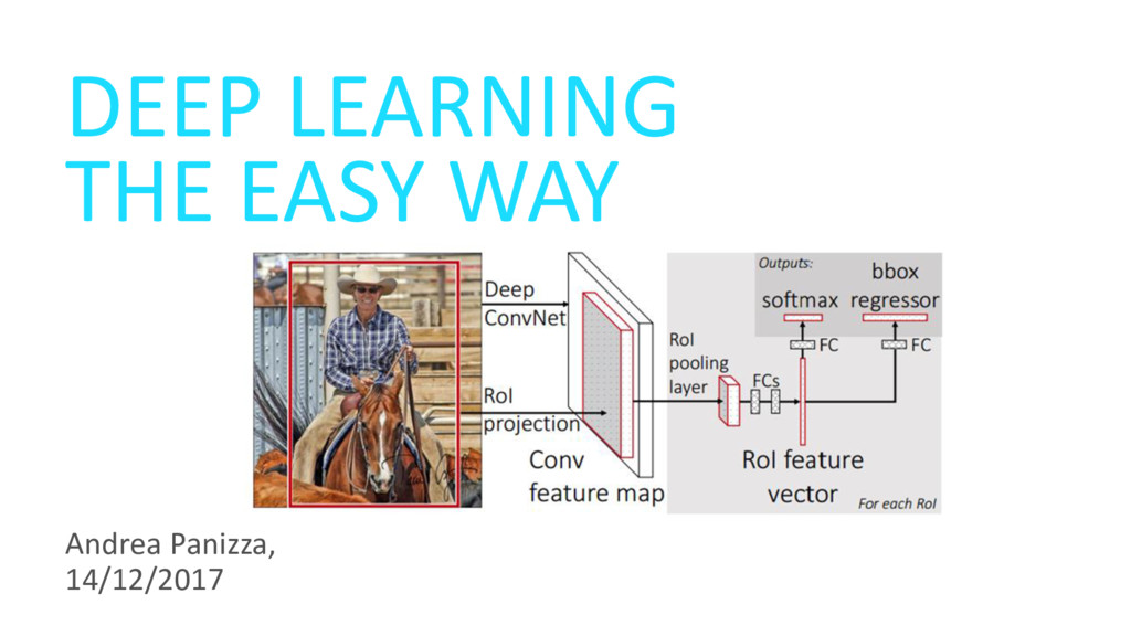
Deep Learning can be understood as a set of tools to efficiently train neural networks with many layers, without overfitting the model to the training set. While a theoretical explanation for the generalization power of large capacity deep neural network is still lacking, the availability of very user-friendly libraries (e.g., Keras,PyTorch, etc.) allows even people without a formal training in Deep Learning to experiment and build performing networks. This presentation will show an application to a simple image classification benchmark.

Transcript

1. DEEP LEARNING THE EASY WAY Andrea Panizza, 14/12/2017
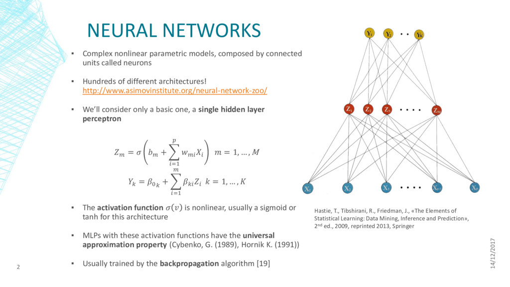
2. NEURAL NETWORKS ▪ Complex nonlinear parametric models, composed by connected units called neurons ▪ Hundreds of different architectures! http://www.asimovinstitute.org/neural-network-zoo/ ▪ We’ll consider only a basic one, a single hidden layer perceptron = + ෍ =1 = 1, … , M = 0 + ෍ =1 = 1, … , ▪ The activation function is nonlinear, usually a sigmoid or tanh for this architecture ▪ MLPs with these activation functions have the universal approximation property (Cybenko, G. (1989), Hornik K. (1991)) ▪ Usually trained by the backpropagation algorithm [19] 14/12/2017 2 Hastie, T., Tibshirani, R., Friedman, J., «The Elements of Statistical Learning: Data Mining, Inference and Prediction», 2nd ed., 2009, reprinted 2013, Springer
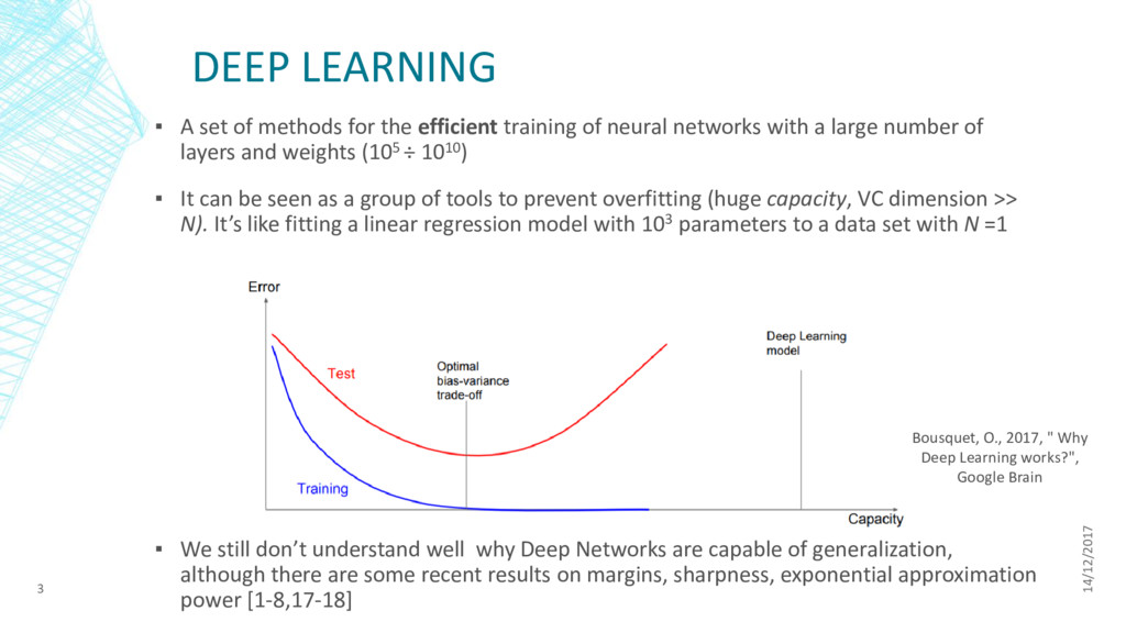
3. DEEP LEARNING ▪ A set of methods for the efficient training of neural networks with a large number of layers and weights (105 ÷ 1010) ▪ It can be seen as a group of tools to prevent overfitting (huge capacity, VC dimension >> N). It’s like fitting a linear regression model with 103 parameters to a data set with N =1 ▪ We still don’t understand well why Deep Networks are capable of generalization, although there are some recent results on margins, sharpness, exponential approximation power [1-8,17-18] 14/12/2017 3 Bousquet, O., 2017, " Why Deep Learning works?", Google Brain
4. DEEP NEURAL NETWORKS ▪ Usually (but not necessarily) trained on huge data sets ▪ DNNs have revolutionized Machine Learning, offering a unified approach to problems which up to 10 years ago were dealt with in completely different ways: ➢Speech recognition [9] ➢Computer vision (better-than-human performance on some tasks) [10] ➢Natural language processing [11] 14/12/2017 4
5. DEEP NEURAL NETWORKS ▪ Training and making predictions with DNN required the introduction of new hardware (GPU), new regularization methods, new activation functions and new approaches to optimization ▪ The lack of a general theory guiding the choice of the best architecture, is partly compensated by the availability of very user-friendly libraries (e.g., Keras,PyTorch, etc.) which allow even people without a formal training in Deep Learning to experiment and build performing networks ▪ I will introduce DNNs for image classification, with an application to a classic benchmark 14/12/2017 5
6. CONVOLUTIONAL NEURAL NETWORKS ▪ Born in the ‘90 [12], but brought to fame by the excellent paper by Krizhevsky, Sutskever e Hinton [13]. Goal: image classification ▪ Before the introduction of CNN, complex algorithms were used to identify low-level features (edges, corners, blobs, etc.) in the image, and combine them to obtain high-level features, which were then ordered in a vector and passed as input to a traditional classification algorithm (e.g., logistic regression or LDA) ▪ CNNs learn features automatically: each layer learns gradually more complex features, while the output layer performs the classification. A single algorithm for the whole image classification process 14/12/2017 6
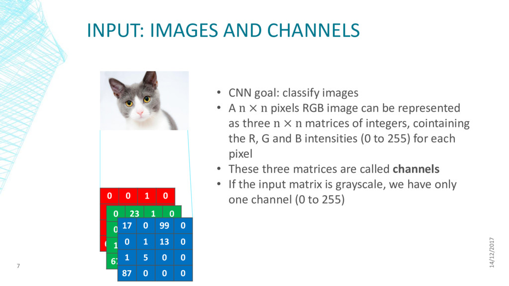
7. INPUT: IMAGES AND CHANNELS 14/12/2017 7 • CNN goal: classify images • A n × n pixels RGB image can be represented as three n × n matrices of integers, cointaining the R, G and B intensities (0 to 255) for each pixel • These three matrices are called channels • If the input matrix is grayscale, we have only one channel (0 to 255) 0 0 1 0 0 1 13 0 1 5 0 0 67 0 0 0 0 23 1 0 0 1 13 0 1 5 0 0 67 0 0 0 17 0 99 0 0 1 13 0 1 5 0 0 87 0 0 0
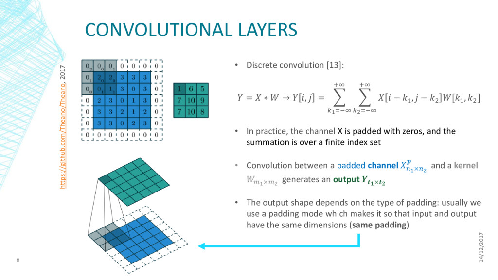
8. CONVOLUTIONAL LAYERS 14/12/2017 8 https://github.com/Theano/Theano, 2017 • Discrete convolution [13]: = ∗ → , = ෍ 1=−∞ +∞ ෍ 2=−∞ +∞ − 1 , − 2 [1 , 2 ] • In practice, the channel X is padded with zeros, and the summation is over a finite index set • Convolution between a padded channel 1×2 and a kernel 1×2 generates an output × • The output shape depends on the type of padding: usually we use a padding mode which makes it so that input and output have the same dimensions (same padding)
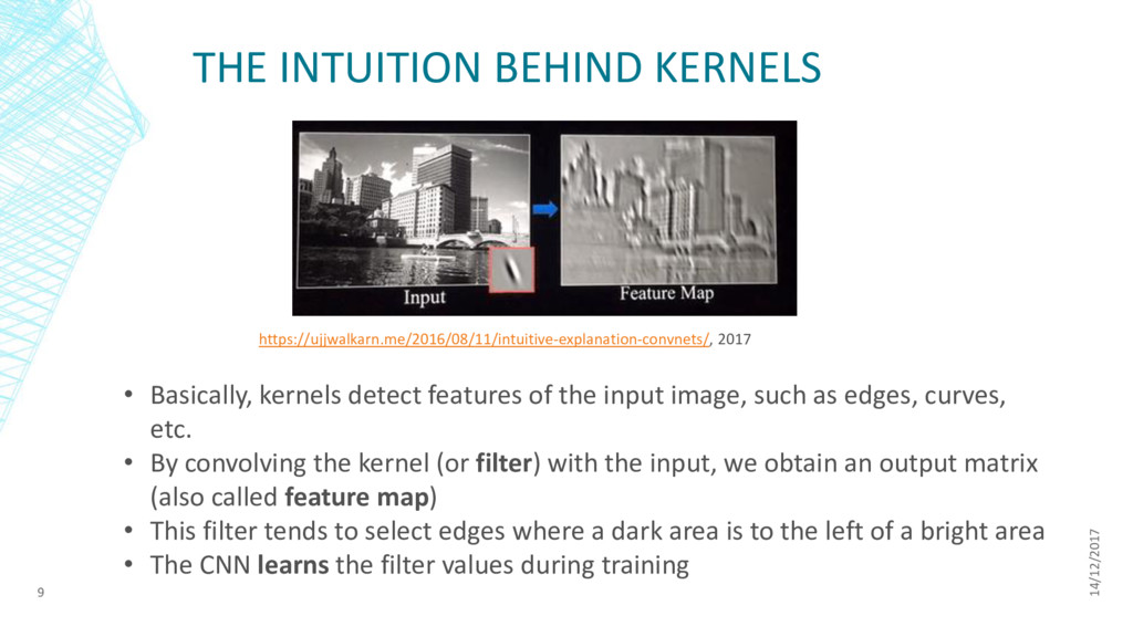
9. THE INTUITION BEHIND KERNELS 14/12/2017 9 https://ujjwalkarn.me/2016/08/11/intuitive-explanation-convnets/, 2017 • Basically, kernels detect features of the input image, such as edges, curves, etc. • By convolving the kernel (or filter) with the input, we obtain an output matrix (also called feature map) • This filter tends to select edges where a dark area is to the left of a bright area • The CNN learns the filter values during training
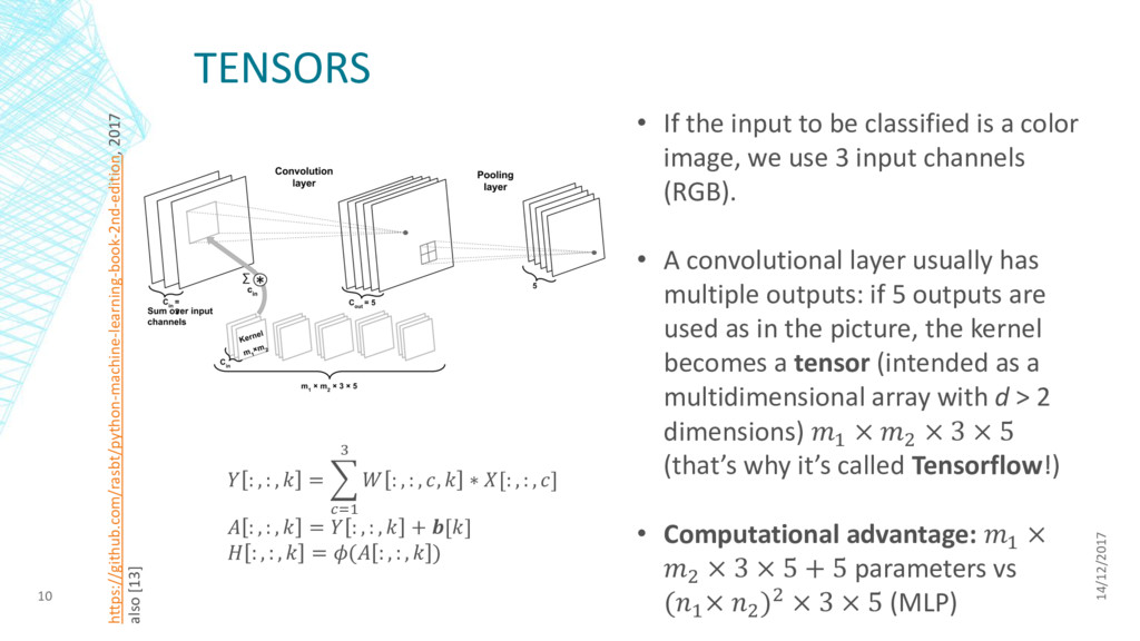
10. TENSORS 14/12/2017 10 • If the input to be classified is a color image, we use 3 input channels (RGB). • A convolutional layer usually has multiple outputs: if 5 outputs are used as in the picture, the kernel becomes a tensor (intended as a multidimensional array with d > 2 dimensions) 1 × 2 × 3 × 5 (that’s why it’s called Tensorflow!) • Computational advantage: 1 × 2 × 3 × 5 + 5 parameters vs (1 × 2 )2 × 3 × 5 (MLP) https://github.com/rasbt/python-machine-learning-book-2nd-edition, 2017 also [13] : , : , = ෍ =1 3 : , : , , ∗ [: , : , ] : , : , = : , : , + [] : , : , = ( : , : , )
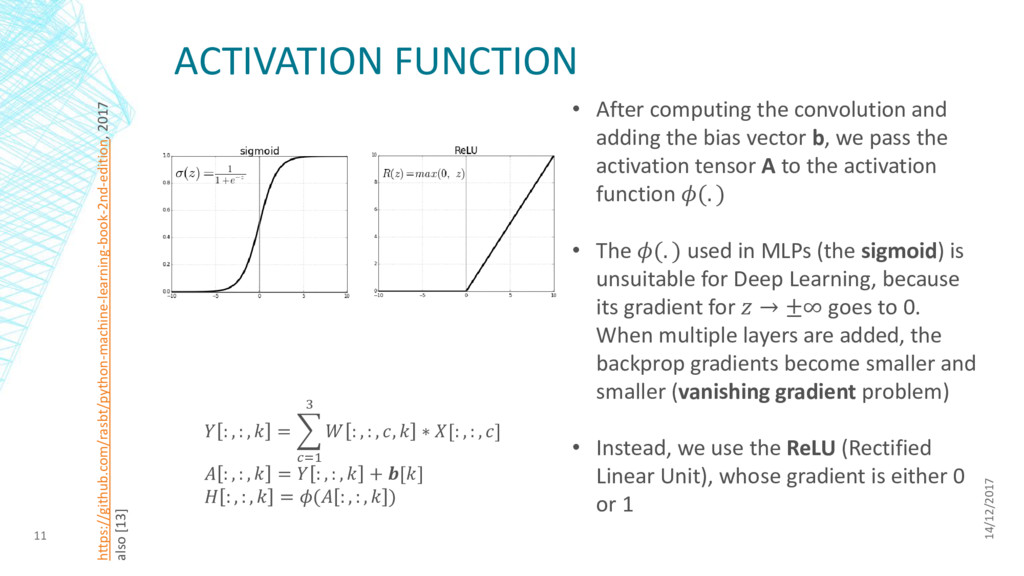
11. ACTIVATION FUNCTION 14/12/2017 11 • After computing the convolution and adding the bias vector b, we pass the activation tensor A to the activation function (. ) • The (. ) used in MLPs (the sigmoid) is unsuitable for Deep Learning, because its gradient for → ±∞ goes to 0. When multiple layers are added, the backprop gradients become smaller and smaller (vanishing gradient problem) • Instead, we use the ReLU (Rectified Linear Unit), whose gradient is either 0 or 1 https://github.com/rasbt/python-machine-learning-book-2nd-edition, 2017 also [13] : , : , = ෍ =1 3 : , : , , ∗ [: , : , ] : , : , = : , : , + [] : , : , = ( : , : , )
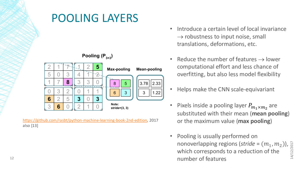
12. POOLING LAYERS 14/12/2017 12 • Introduce a certain level of local invariance  robustness to input noise, small translations, deformations, etc. • Reduce the number of features  lower computational effort and less chance of overfitting, but also less model flexibility • Helps make the CNN scale-equivariant • Pixels inside a pooling layer 1×2 are substituted with their mean (mean pooling) or the maximum value (max pooling) • Pooling is usually performed on nonoverlapping regions (stride = (1 , 2 )), which corresponds to a reduction of the number of features https://github.com/rasbt/python-machine-learning-book-2nd-edition, 2017 also [13]
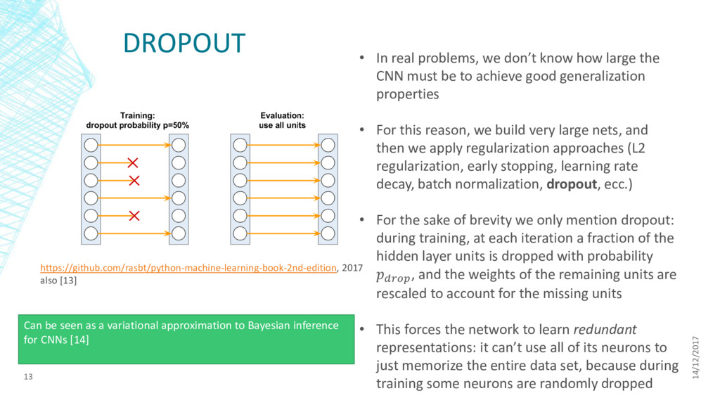
13. DROPOUT 14/12/2017 13 • In real problems, we don’t know how large the CNN must be to achieve good generalization properties • For this reason, we build very large nets, and then we apply regularization approaches (L2 regularization, early stopping, learning rate decay, batch normalization, dropout, ecc.) • For the sake of brevity we only mention dropout: during training, at each iteration a fraction of the hidden layer units is dropped with probability , and the weights of the remaining units are rescaled to account for the missing units • This forces the network to learn redundant representations: it can’t use all of its neurons to just memorize the entire data set, because during training some neurons are randomly dropped Can be seen as a variational approximation to Bayesian inference for CNNs [14] https://github.com/rasbt/python-machine-learning-book-2nd-edition, 2017 also [13]
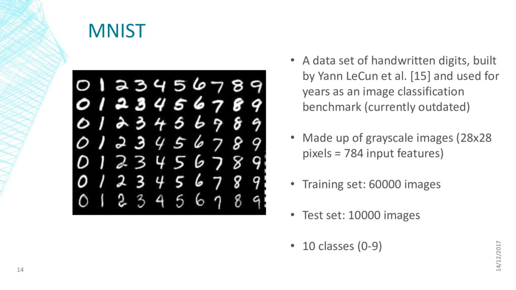
14. MNIST 14/12/2017 14 • A data set of handwritten digits, built by Yann LeCun et al. [15] and used for years as an image classification benchmark (currently outdated) • Made up of grayscale images (28x28 pixels = 784 input features) • Training set: 60000 images • Test set: 10000 images • 10 classes (0-9)
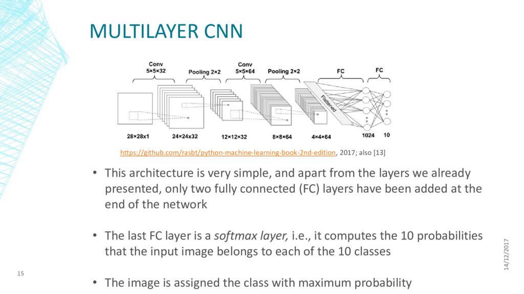
15. MULTILAYER CNN 14/12/2017 15 • This architecture is very simple, and apart from the layers we already presented, only two fully connected (FC) layers have been added at the end of the network • The last FC layer is a softmax layer, i.e., it computes the 10 probabilities that the input image belongs to each of the 10 classes • The image is assigned the class with maximum probability https://github.com/rasbt/python-machine-learning-book-2nd-edition, 2017; also [13]
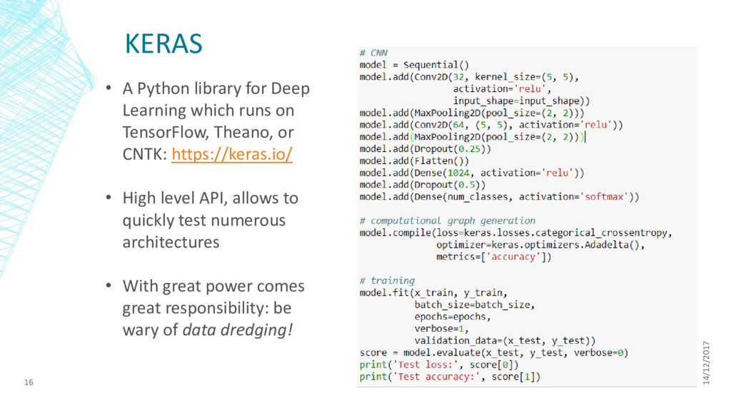
16. KERAS 14/12/2017 16 • A Python library for Deep Learning which runs on TensorFlow, Theano, or CNTK: https://keras.io/ • High level API, allows to quickly test numerous architectures • With great power comes great responsibility: be wary of data dredging!
17. RESULTS 14/12/2017 17 • 21 minutes training on an i7 laptop 8 Gb (12 epochs) • Accuracy on training set: 99.35 % • Accuracy on test set: 99.33% (only 67 misclassified images out of 10000) • Not only the CNN is simple and accurate, but also the fact that the accuracy on training and test set are so similar, strongly suggests that we neither underfit or overfit the training set • In the ’00, you would have to struggle much more on more powerful hardware, for a meager 95%!
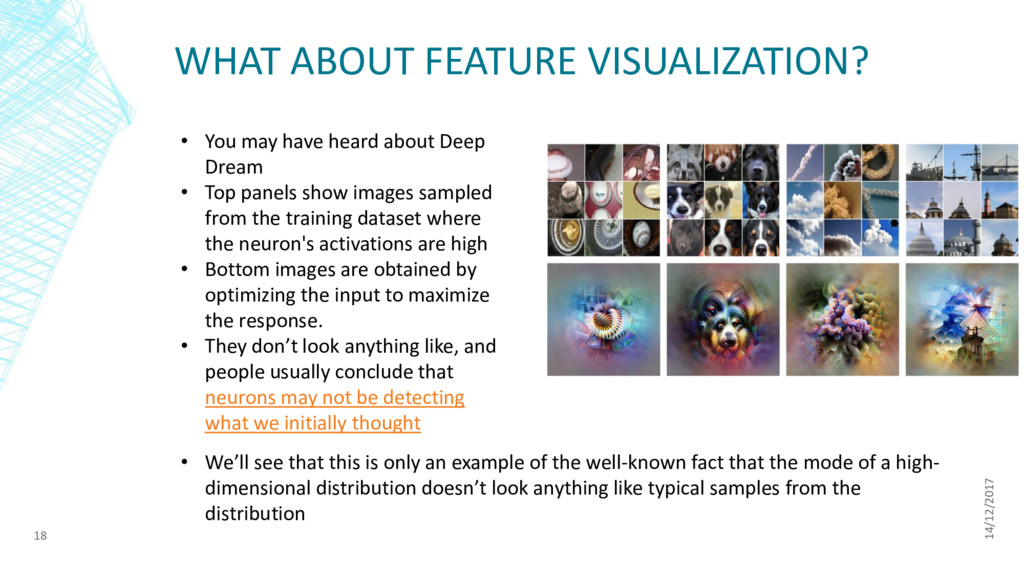
18. WHAT ABOUT FEATURE VISUALIZATION? 14/12/2017 18 • You may have heard about Deep Dream • Top panels show images sampled from the training dataset where the neuron's activations are high • Bottom images are obtained by optimizing the input to maximize the response. • They don’t look anything like, and people usually conclude that neurons may not be detecting what we initially thought • We’ll see that this is only an example of the well-known fact that the mode of a high- dimensional distribution doesn’t look anything like typical samples from the distribution
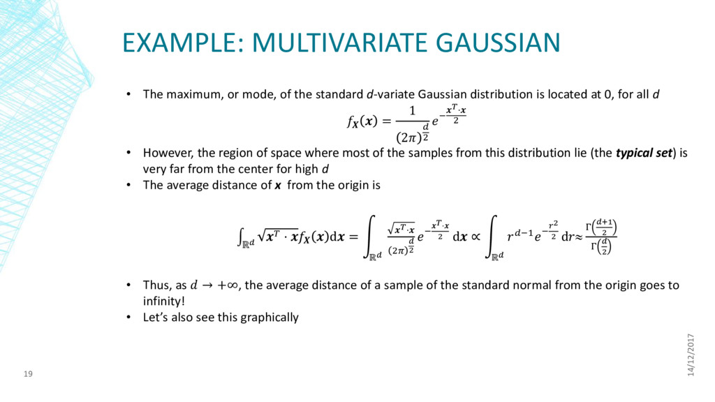
19. EXAMPLE: MULTIVARIATE GAUSSIAN 14/12/2017 19 • The maximum, or mode, of the standard d-variate Gaussian distribution is located at 0, for all d = 1 2 2 − ⋅ 2 • However, the region of space where most of the samples from this distribution lie (the typical set) is very far from the center for high d • The average distance of x from the origin is ධ ℝ ⋅ d = ඲ ℝ ⋅ 2 2 −⋅ 2 d ∝ ඲ ℝ −1−2 2 d Γ +1 2 Γ 2 • Thus, as → +∞, the average distance of a sample of the standard normal from the origin goes to infinity! • Let’s also see this graphically
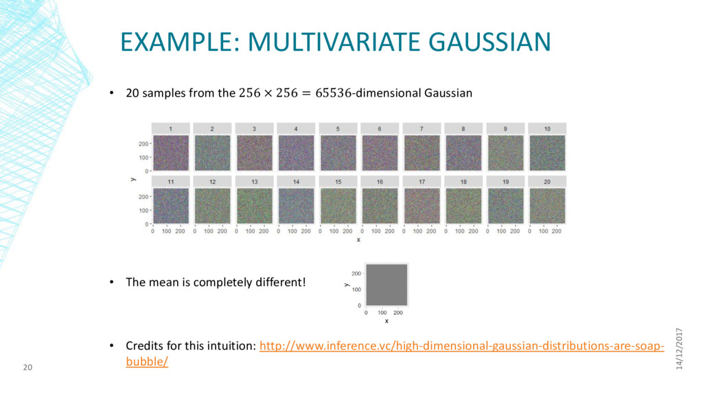
20. EXAMPLE: MULTIVARIATE GAUSSIAN 14/12/2017 20 • 20 samples from the 256 × 256 = 65536-dimensional Gaussian • The mean is completely different! • Credits for this intuition: http://www.inference.vc/high-dimensional-gaussian-distributions-are-soap- bubble/
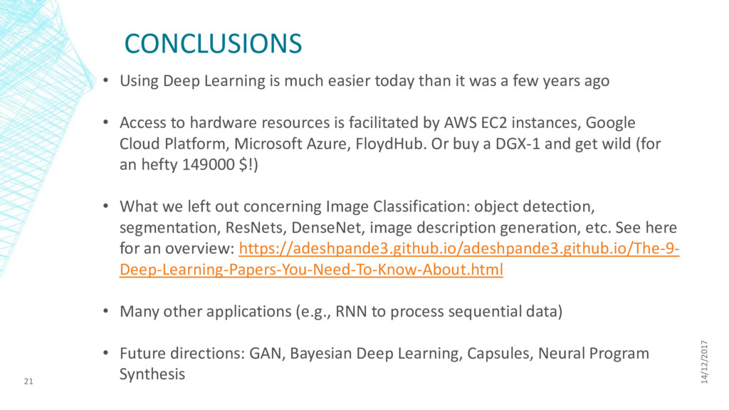
21. CONCLUSIONS 14/12/2017 21 • Using Deep Learning is much easier today than it was a few years ago • Access to hardware resources is facilitated by AWS EC2 instances, Google Cloud Platform, Microsoft Azure, FloydHub. Or buy a DGX-1 and get wild (for an hefty 149000 $!) • What we left out concerning Image Classification: object detection, segmentation, ResNets, DenseNet, image description generation, etc. See here for an overview: https://adeshpande3.github.io/adeshpande3.github.io/The-9- Deep-Learning-Papers-You-Need-To-Know-About.html • Many other applications (e.g., RNN to process sequential data) • Future directions: GAN, Bayesian Deep Learning, Capsules, Neural Program Synthesis
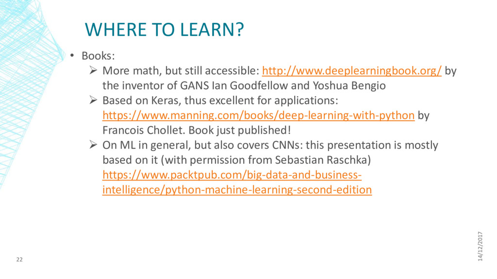
22. WHERE TO LEARN? 14/12/2017 22 • Books: ➢ More math, but still accessible: http://www.deeplearningbook.org/ by the inventor of GANS Ian Goodfellow and Yoshua Bengio ➢ Based on Keras, thus excellent for applications: https://www.manning.com/books/deep-learning-with-python by Francois Chollet. Book just published! ➢ On ML in general, but also covers CNNs: this presentation is mostly based on it (with permission from Sebastian Raschka) https://www.packtpub.com/big-data-and-business- intelligence/python-machine-learning-second-edition
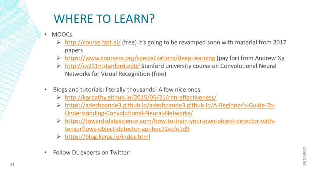
23. WHERE TO LEARN? 14/12/2017 23 • MOOCs: ➢ http://course.fast.ai/ (free) it’s going to be revamped soon with material from 2017 papers ➢ https://www.coursera.org/specializations/deep-learning (pay for) from Andrew Ng ➢ http://cs231n.stanford.edu/ Stanford university course on Convolutional Neural Networks for Visual Recognition (free) • Blogs and tutorials: literally thousands! A few nice ones: ➢ http://karpathy.github.io/2015/05/21/rnn-effectiveness/ ➢ https://adeshpande3.github.io/adeshpande3.github.io/A-Beginner's-Guide-To- Understanding-Convolutional-Neural-Networks/ ➢ https://towardsdatascience.com/how-to-train-your-own-object-detector-with- tensorflows-object-detector-api-bec72ecfe1d9 ➢ https://blog.keras.io/index.html • Follow DL experts on Twitter!
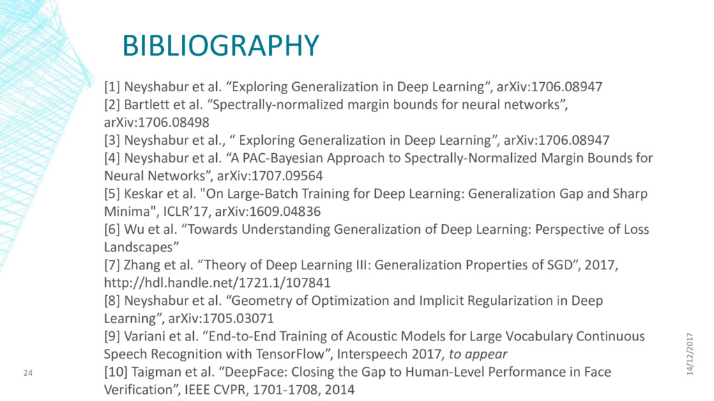
24. BIBLIOGRAPHY 14/12/2017 24 [1] Neyshabur et al. “Exploring Generalization in Deep Learning”, arXiv:1706.08947 [2] Bartlett et al. “Spectrally-normalized margin bounds for neural networks”, arXiv:1706.08498 [3] Neyshabur et al., “ Exploring Generalization in Deep Learning”, arXiv:1706.08947 [4] Neyshabur et al. “A PAC-Bayesian Approach to Spectrally-Normalized Margin Bounds for Neural Networks”, arXiv:1707.09564 [5] Keskar et al. "On Large-Batch Training for Deep Learning: Generalization Gap and Sharp Minima", ICLR’17, arXiv:1609.04836 [6] Wu et al. “Towards Understanding Generalization of Deep Learning: Perspective of Loss Landscapes” [7] Zhang et al. “Theory of Deep Learning III: Generalization Properties of SGD”, 2017, http://hdl.handle.net/1721.1/107841 [8] Neyshabur et al. “Geometry of Optimization and Implicit Regularization in Deep Learning”, arXiv:1705.03071 [9] Variani et al. “End-to-End Training of Acoustic Models for Large Vocabulary Continuous Speech Recognition with TensorFlow”, Interspeech 2017, to appear [10] Taigman et al. “DeepFace: Closing the Gap to Human-Level Performance in Face Verification”, IEEE CVPR, 1701-1708, 2014
25. BIBLIOGRAPHY 14/12/2017 25 [11] Wu et al. “Google's Neural Machine Translation System: Bridging the Gap between Human and Machine Translation”, arXiv:1609.08144 [12] LeCun et al. " Handwritten Digit Recognition with a Back-Propagation Network ", NIPS conference, 1989 [13] Krizhevsky et al. “ImageNet Classification with Deep Convolutional Neural Networks”, NIPS conference, 2012 [14] Raschka and Mirjalili «Python Machine Learning», 2nd ed., Packt, 2017 [15] Gal and Ghahramani, «Bayesian Convolutional Neural Networks with Bernoulli Approximate Variational Inference”, NIPS conference, 2015 [16] LeCun et al. “Gradient-Based Learning Applied to Document Recognition”, Proceedings of the IEEE, 86(11): 2278-2324, 1998 [17] Shiyu & Srikant “ Why deep neural networks for function approximation?”, ICLR 2017 [18] Khrulkov et al. “Expressive power of recurrent neural networks”, https://arxiv.org/abs/1711.00811 [19] Rumelhart, David E.; Hinton, Geoffrey E.; Williams, Ronald J. (8 October 1986). "Learning representations by back-propagating errors". Nature. 323 (6088): 533–536.