Computer Vision Project 3: SLAM

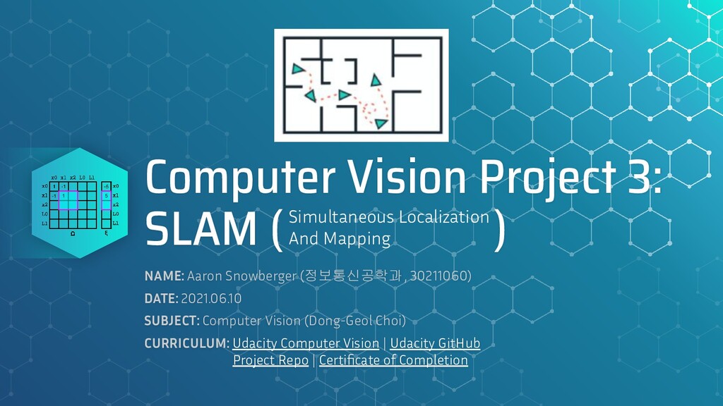
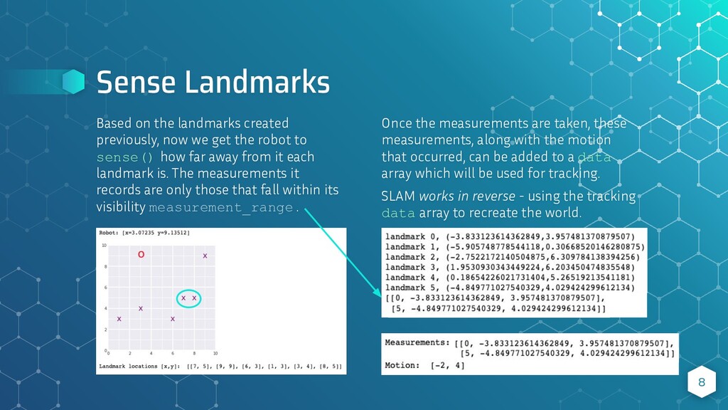
SLAM stands for Simultaneous Localization And Mapping. As a part of Udacity's Computer Vision Nanodegree, I generated a random world with randomly placed landmarks, and made a robot perform random movements within that world. Measurements between the robot location and nearby landmarks were performed at each step, and using the robot's motion, and measurements to the landmarks, its location was tracked over time.

This PPT was submitted as a part of my PhD coursework to detail my project process and reflection.

Transcript

1. Computer Vision Project 3:
   SLAM ( )
   NAME: Aaron Snowberger (정보통신공학과, 30211060)
   DATE: 2021.06.10
   SUBJECT: Computer Vision (Dong-Geol Choi)
   CURRICULUM: Udacity Computer Vision | Udacity GitHub
   Project Repo | Certificate of Completion
   Simultaneous Localization
   And Mapping
   

   View Slide

2. CONTENTS
   01 Problem Overview
   02 Setting up the World
   a. Robot Class
   b. Visualize the World
   c. Sense Landmarks
   d. Constraint Matrices, 𝝮 & 𝝽 (#1-5)
   e. Motion Constraints
   03 Implement (Graph) SLAM
   a. Generate Environment & data
   b. Initialize Constraints
   c. Update measurements
   d. Run SLAM & Visualize results
   e. Visualize the World
   04 Test Model Accuracy
   05 Project Reflection
   06 Conclusion & Future Research
   2
   SLAM: Simultaneous
   Localization And Mapping
   The idea is to detect the
   motion of a robot in an
   environment by tracking
   measurements from its
   sensors over time.
   (A similar concept to how
   a self-driving car works.)
   

   View Slide

3. Problem Overview
   To track the motion of a robot from sensor readings
   1
   

   View Slide

4. Problem Overview
   In this project, I set up a 2-dimensional world and perform SLAM
   (Simultaneous Localization And Mapping) on a robot in order to track
   its location and recreate a map of the environment based on the
   robot’s motion and sensor measurements of landmarks over time.
   In order to do this, a square matrix (𝝮) and a vector (𝝽) are used to
   track all robot poses (xi) and landmark locations (Li).
   Since this localization and map-building relies on the visual sensing of landmarks, this is a computer vision problem. 4
   

   View Slide

5. Setting up the World
   Build 2D world and the robot with initial position &
   measurements of uncertainty
   2
   

   View Slide

6. Apart from instantiating a new instance of the Robot and initializing its internal variables
   based on the parameters that are passed in, there are three important methods as well.
   Robot Class
   make_landmarks(num)
   :
   Creates a given number of
   randomly located landmarks by
   selecting a random x and
   random y location within the
   world_size
   6
   move(dx, dy):
   Attempts to move the robot by
   delta x (dx) and delta y (dy). If
   outside the world boundary,
   then nothing happens and the
   function returns failure.
   This function also includes
   motion_noise which is a
   small random value between
   [-1.0, 1.0] that accounts for data
   loss recorded by motion sensors
   as the robot moves around the
   environment.
   sense():
   Computes dx and dy distances
   to landmarks (referencing
   internal variables it keeps track
   of, i.e. self.landmarks)
   within the visibility range and
   returns the landmark index
   along with the measurements.
   This function also includes
   measurement_noise which is
   a small random value between
   [-1.0, 1.0] that accounts for data
   loss in landmark measurements.
   

   View Slide

7. Visualize the World
   Instantiate the Robot Class with
   some small values just to visualize
   it (later it will be 10x bigger).
   7
   r.move(-2, 4) #(x,y)
   r.make_landmarks (6)
   display_world(*args)
   

   View Slide

8. Once the measurements are taken, these
   measurements, along with the motion
   that occurred, can be added to a data
   array which will be used for tracking.
   SLAM works in reverse - using the tracking
   data array to recreate the world.
   Sense Landmarks
   Based on the landmarks created
   previously, now we get the robot to
   sense() how far away from it each
   landmark is. The measurements it
   records are only those that fall within its
   visibility measurement_range .
   8
   

   View Slide

9. Constraint Matrices, Omega (𝝮) & Xi (𝝽) #1
   9
   The constraint matrix 𝝮 keeps track of
   the relationships between each robot
   location and the landmarks it detects.
   x represents the position of the robot
   (in one-dimensional space).
   L represents the landmarks it detects.
   Motion Constraints
   The robot moves 5 steps from x0 → x1:
   x1 = x0 + 5
   x0 - x1 = -5
   x1 - x0 = 5
   

   View Slide

10. Constraint Matrices, Omega (𝝮) & Xi (𝝽) #2
    10
    The constraint matrix 𝝮 keeps track of
    the relationships between each robot
    location and the landmarks it detects.
    x represents the position of the robot
    (in one-dimensional space).
    L represents the landmarks it detects.
    Motion Constraints
    The robot moves -4 steps from x1 → x2:
    x2 = x1 - 4
    x1 - x2 = (original 5) + 4 = 9
    x2 - x1 = -4
    -4
    9
    2 -1
    -1 1
    

    View Slide

11. Constraint Matrices, Omega (𝝮) & Xi (𝝽) #3
    11
    The constraint matrix 𝝮 keeps track of
    the relationships between each robot
    location and the landmarks it detects.
    x represents the position of the robot
    (in one-dimensional space).
    L represents the landmarks it detects.
    Measurement Constraints
    The robot detects landmark L0 @ x1 and
    measures it to be 9 steps away:
    This means the 4 intersections of:
    (x1,x1), (x1,L0), (L0,x1), (L0,L0)
    must be updated.
    x1: L0 distance = 9
    x1 - L0 = -9
    L0 - x1 = 9
    0
    3 -1
    -1 1 9
    

    View Slide

12. Constraint Matrices, Omega (𝝮) & Xi (𝝽) #4
    12
    The constraint matrix 𝝮 keeps track of
    the relationships between each robot
    location and the landmarks it detects.
    x represents the position of the robot
    (in one-dimensional space).
    L represents the landmarks it detects.
    Measurement Constraints
    The robot detects landmark L0 @ x1 and
    measures it to be 9 steps away:
    This means the 4 intersections of:
    (x1,x1), (x1,L0), (L0,x1), (L0,L0)
    must be updated.
    x2: L0 distance = -3, L1 distance = 7
    x2 - L0 = 3 x2 - L1 = -7
    L0 - x2 = -3 L1 - x2 = 7
    -1
    -1
    -1 6
    -8
    7
    

    View Slide

13. The best solution for finding all the motion positions and all the
    landmark positions is to multiply the inverse of 𝝮 x 𝝽.
    For 2D space, we can either:
    1. use two 𝝻 = 𝝮-1 x 𝝽 functions (one for x values and one for y)
    2. OR double the size of our matrices (x0, y0, x1, y1, … Lx0, Ly0, Lx1, Ly1)
    Constraint Matrices, Omega (𝝮) & Xi (𝝽) #5
    13
    

    View Slide

14. Implement (Graph) SLAM
    From data, determine the robot’s location
    3
    

    View Slide

15. Generate Environment & data
    make_data()
    generates a
    world grid with
    landmarks and
    places a robot in
    the center of the
    world.
    Then it generates
    motion and
    measurement
    data by moving
    the robot and
    sensing the
    landmarks over
    some number of
    time steps.
    15
    

    View Slide

16. Initialize Constraints (𝝮 & 𝝽)
    For testing purposes,
    we begin with a
    10x10 2D grid with
    only 2 landmarks.
    16
    𝝮 𝝽
    

    View Slide

17. Update Measurements (Implement SLAM)
    slam() takes 6 parameters and returns 𝝻
    1. data - measurements & motions
    collected for a number of time steps
    2. N - number of time steps
    3. num_landmarks - # of landmarks
    4. world_size - size (w/h) of the world
    5. motion_noise - random noise
    associated with motion. Update
    confidence is 1.0/motion_noise
    6. measurement_noise - random noise
    associated with sensing. Update
    weight is 1.0/measurement_noise
    𝝻 is the entire path traversed by the robot
    (all x,y poses) *and* all landmark locations.
    17
    Possibly the most important function is
    the helper function to update the matrices.
    It needs to take into account:
    1. Both indices that must be updated
    2. In both matrices
    3. As well as motion_noise
    4. And measurement_noise
    5. And the delta (difference in x or y)
    

    View Slide

18. Run SLAM (𝝻 = 𝝮-1 x 𝝽)
    18
    𝝮-1 *𝝽 =𝝻
    

    View Slide

19. Visualize the World
    The difference between the robot’s
    estimated final position and its true
    final position is:
    dx = 8.24910 - 9.52082 = -1.27172
    dy = 7.35233 - 6.98117 = 0.37116
    Total = 1.32478 ( )
    And estimated landmark positions are
    close to the true landmark positions,
    so our implementation works well! 19
    

    View Slide

20. Test Model Accuracy
    How closely do our predictions match reality?
    4
    

    View Slide

21. Test Case 1
    21
    Test Case 2
    The more closely my results match the results from the
    “official answer results,” the better my algorithm is.
    

    View Slide

22. Project Reflection
    Complex simplicity OR simple complexity
    5
    

    View Slide

23. Kalman Filter: keeps track of
    the estimated state of the
    system and uncertainty of the
    estimated event. It is a recursive
    iterator and consists of two
    steps: Predict and Update.
    Baye’s Rule, Gaussian Distributions, & Kalman Filters
    In working on this project, I
    was introduced to many
    new concepts that helped
    me understand how
    prediction models work in
    AI and robotics.
    Baye’s Rule: addresses the
    probability of an event, based
    on initial data & collecting more
    data to improve the probability
    Gaussian: addresses the
    uncertainty related to an
    event’s probability
    23
    

    View Slide

24. Kalman Filter & Graph SLAM Notes
    24
    Graph SLAM: uses information
    matrices that (𝝮 & 𝝽) that are
    generated with a factor graph of
    interdependent observations (two
    observations are related if they
    contain information about the
    same landmark) in order to
    perform Simultaneous
    Localization And Mapping (SLAM).
    

    View Slide

25. Conclusion & Future Research
    Mapping, Sensing, Predicting
    6
    

    View Slide

26. Kalman Filter uses & SLAM Algorithms
    SLAM in a nutshell (Wikipedia)
    Given a series of controls u
    t
    and sensor
    observations o
    t
    over a discrete number of time
    steps t, compute an estimate of the agent’s
    state x
    t
    and a map of the environment m
    t
    .
    With Baye’s Rule:
    Sequentially:
    Future Research needs to be done into
    both additional uses for the Kalman
    Filter, as well as more in-depth research
    into the various other SLAM algorithms.
    SLAM itself is a broad topic and has
    many wide uses including ➀ self-driving
    cars, ➁ unmanned aerial vehicles,
    ➂ autonomous underwater vehicles,
    ➃ planetary rovers, and ➄ robotics.
    Therefore, there are many approaches to
    address this problem, and much to
    explore in many different domains.
    The Kalman Filter is one approach (also
    known as EFK SLAM in robotics), but
    additionally, Acoustic SLAM, Audio-Visual
    SLAM, Collaborative SLAM, FastSLAM,
    Graph SLAM (studied in this project),
    SLAM with DATMO, Active SLAM, and
    RatSLAM to name a few.
    26
    

    View Slide

27. THANKS!
    The Jupyter Notebook used in this project
    including code and output can be found at:
    https://github.com/jekkilekki/computer-vision/tree/
    master/Graph%20SLAM
    27
    

    View Slide