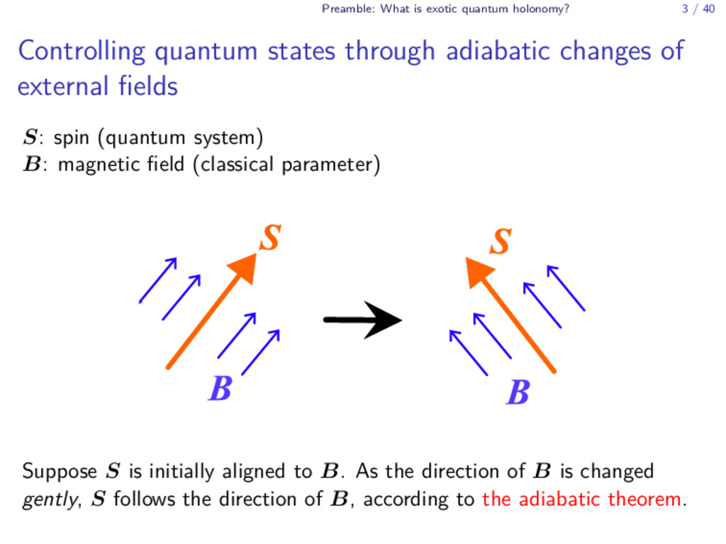
quantum states through adiabatic changes of external fields S: spin (quantum system) B: magnetic field (classical parameter) Suppose S is initially aligned to B. As the direction of B is changed gently, S follows the direction of B, according to the adiabatic theorem.
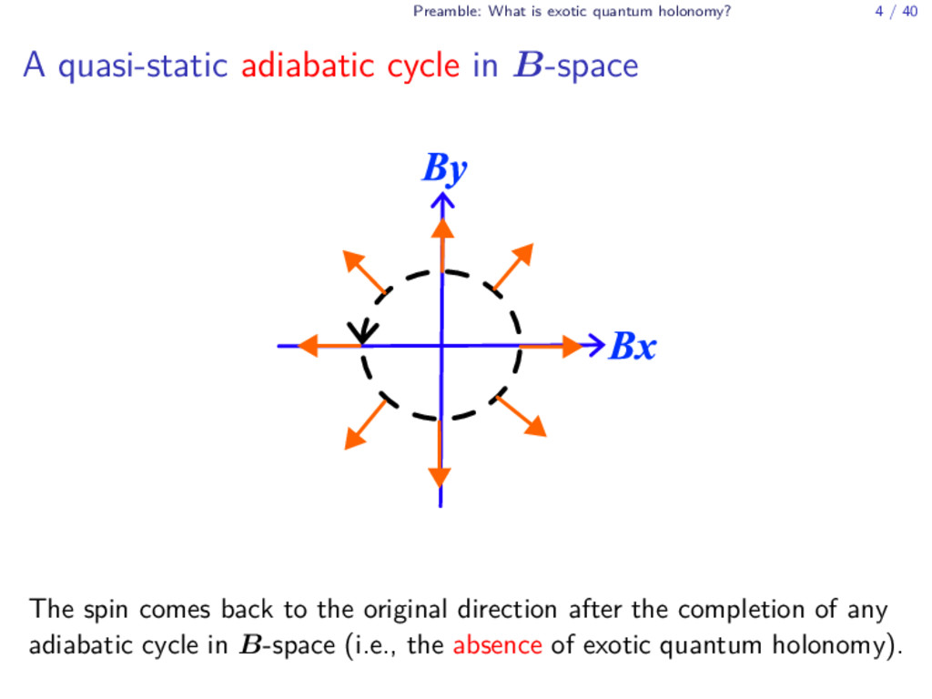
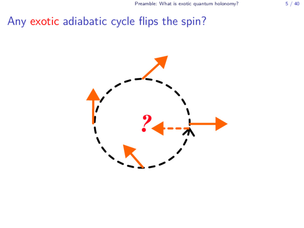
quasi-static adiabatic cycle in B-space The spin comes back to the original direction after the completion of any adiabatic cycle in B-space (i.e., the absence of exotic quantum holonomy).
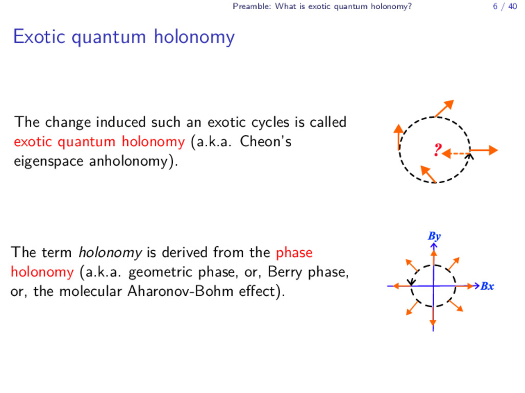
quantum holonomy The change induced such an exotic cycles is called exotic quantum holonomy (a.k.a. Cheon’s eigenspace anholonomy). The term holonomy is derived from the phase holonomy (a.k.a. geometric phase, or, Berry phase, or, the molecular Aharonov-Bohm effect).
I will explain three topics of the exotic quantum holonomy: 1. Examples 2. A topological formulation 3. Classification of adiabatic cycles in non-degenerate two level systems Ref. AT and T. Cheon, Phys. Lett. A 379, 1693 (2015) (or arXiv:1402.1634) and references therein.
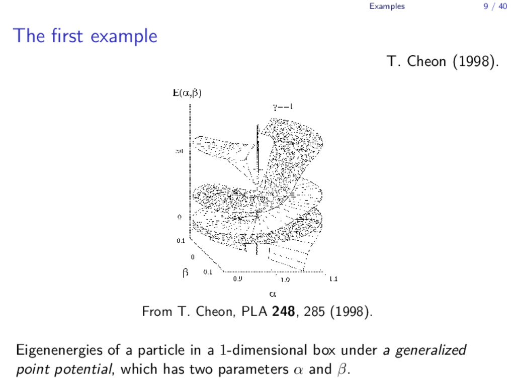
From T. Cheon, PLA 248, 285 (1998). Eigenenergies of a particle in a 1-dimensional box under a generalized point potential, which has two parameters α and β.
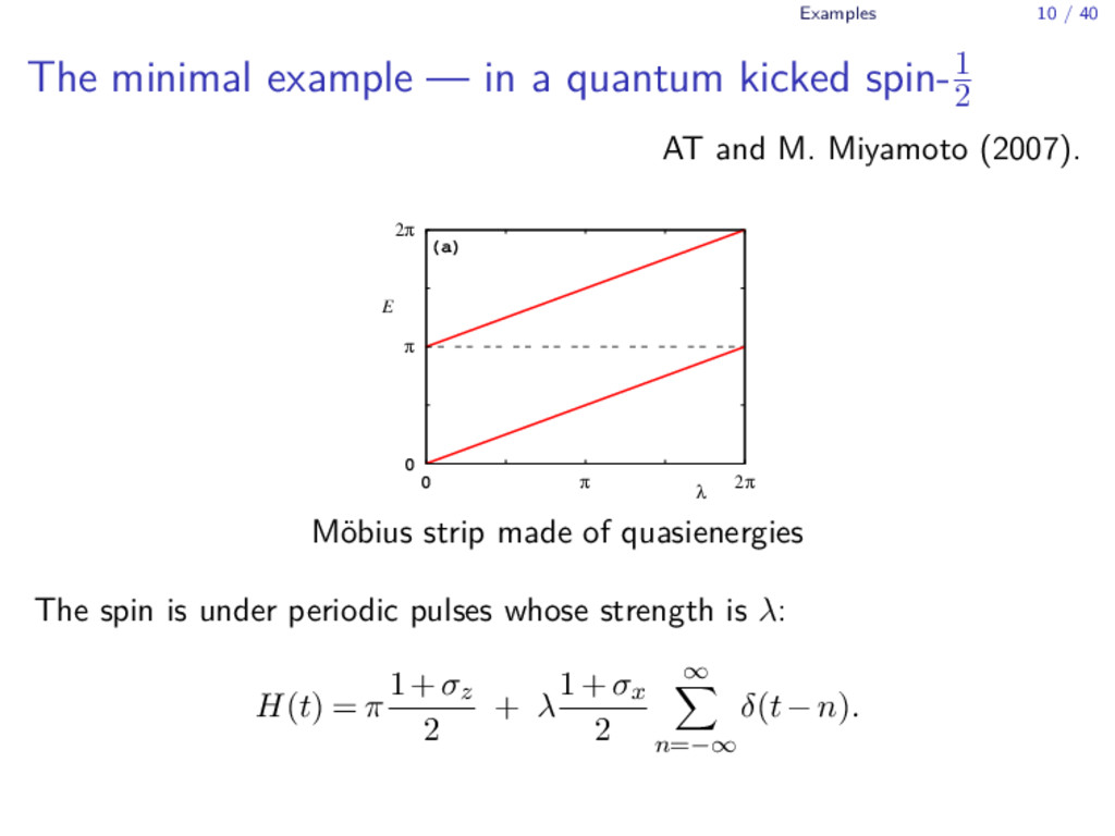
quantum kicked spin-1 2 AT and M. Miyamoto (2007). 2π π 0 2π π 0 (a) λ E M¨ obius strip made of quasienergies The spin is under periodic pulses whose strength is λ: H(t) = π 1+σz 2 + λ 1+σx 2 ∞ ∑ n=−∞ δ(t−n).
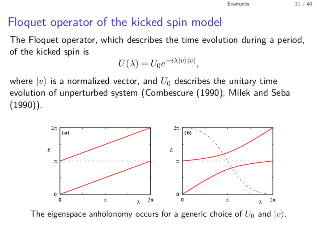
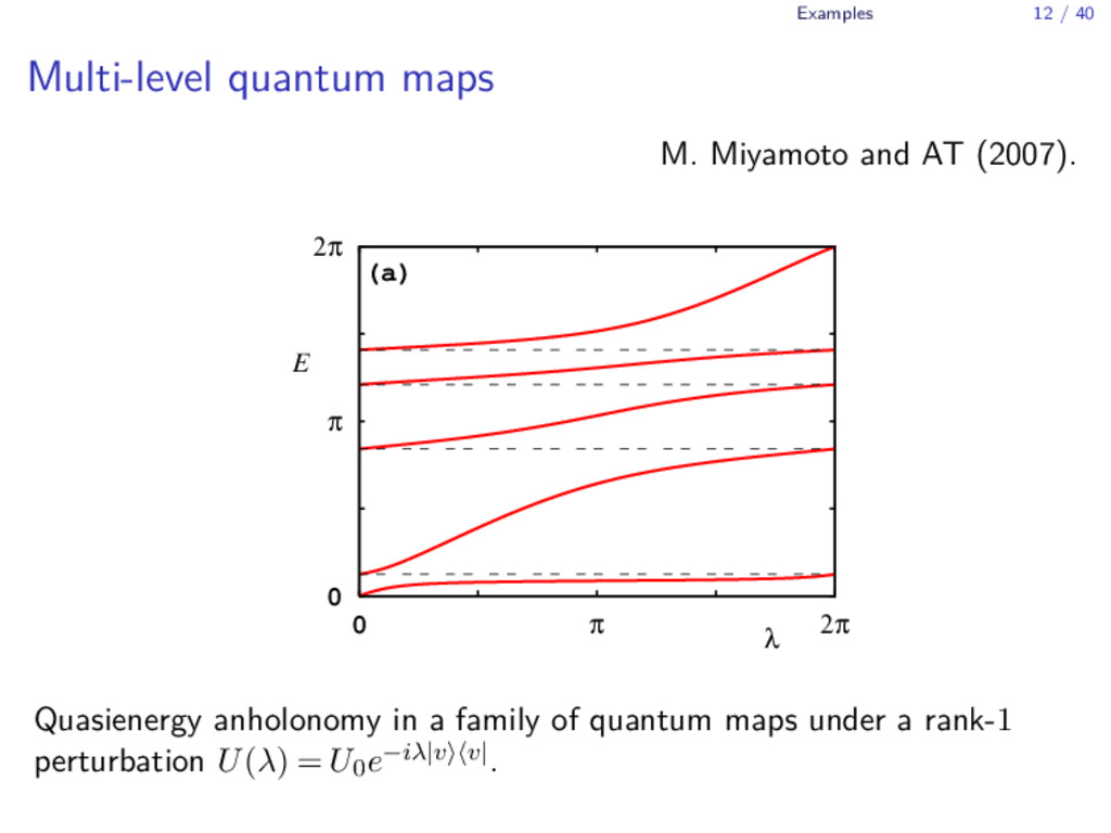
model The Floquet operator, which describes the time evolution during a period, of the kicked spin is U(λ) = U0e−iλ|v⟩⟨v|, where |v⟩ is a normalized vector, and U0 describes the unitary time evolution of unperturbed system (Combescure (1990); Milek and Seba (1990)). 2π π 0 2π π 0 (a) λ E 2π π 0 2π π 0 (b) λ E The eigenspace anholonomy occurs for a generic choice of U0 and |v⟩.
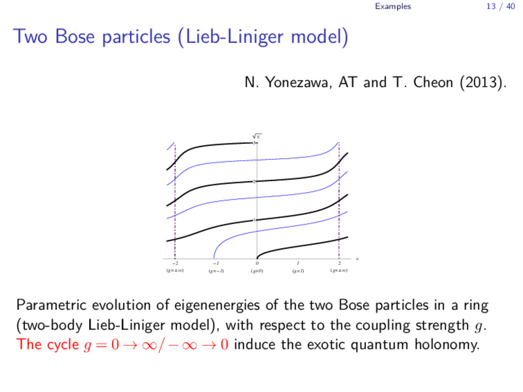
Yonezawa, AT and T. Cheon (2013). 2 g 1 g 1 0 g 0 1 g 1 2 g x 1 2 3 E Parametric evolution of eigenenergies of the two Bose particles in a ring (two-body Lieb-Liniger model), with respect to the coupling strength g. The cycle g = 0 → ∞/−∞ → 0 induce the exotic quantum holonomy.
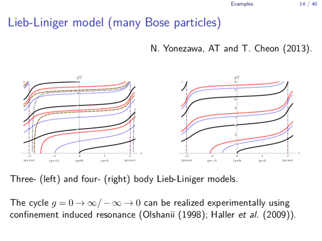
Yonezawa, AT and T. Cheon (2013). 2 g 1 g 1 0 g 0 1 g 1 2 g x 1 2 3 4 5 6 E 2 g 1 g 1 0 g 0 1 g 1 2 g x 1 2 3 4 5 6 7 8 E Three- (left) and four- (right) body Lieb-Liniger models. The cycle g = 0 → ∞/−∞ → 0 can be realized experimentally using confinement induced resonance (Olshanii (1998); Haller et al. (2009)).
Tsutsui, T. F¨ ulop and T. Cheon (2000,2001); S. Ohya (2013,2014)) ▶ Non-Abelian extension (T. Cheon and AT 2009) ▶ Time-dependent Aharonov-Bohm ring (AT and T. Cheon (2010)) ▶ Accelerating adiabatic quantum computation (AT and K. Nemoto (2010)) ▶ Hierarchical many-qubit systems (AT, S. W. Kim and T. Cheon (2011); AT, T. Cheon and S. W. Kim (2012)) ▶ Autonomous Hamiltonians with level crossing (T. Cheon, AT and S. W. Kim, (2009)) ▶ Another good example? (e.g., experimentally feasible ones)
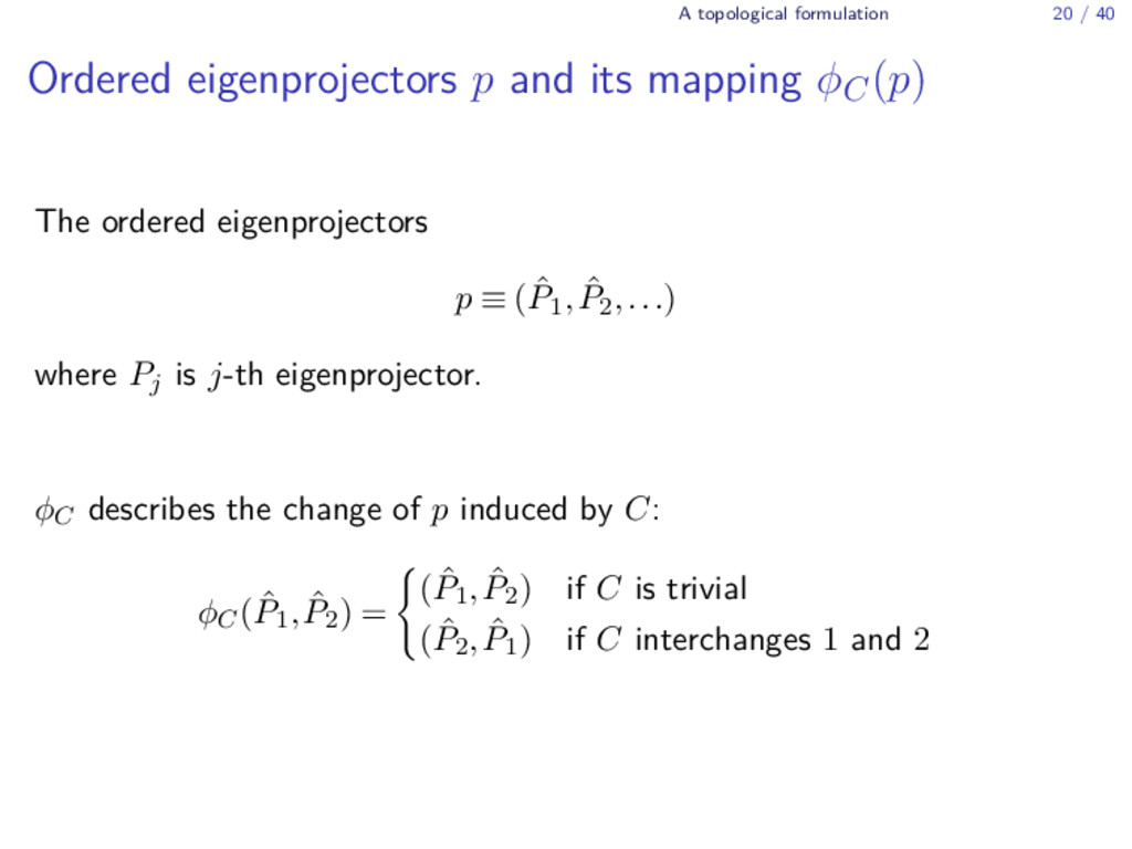
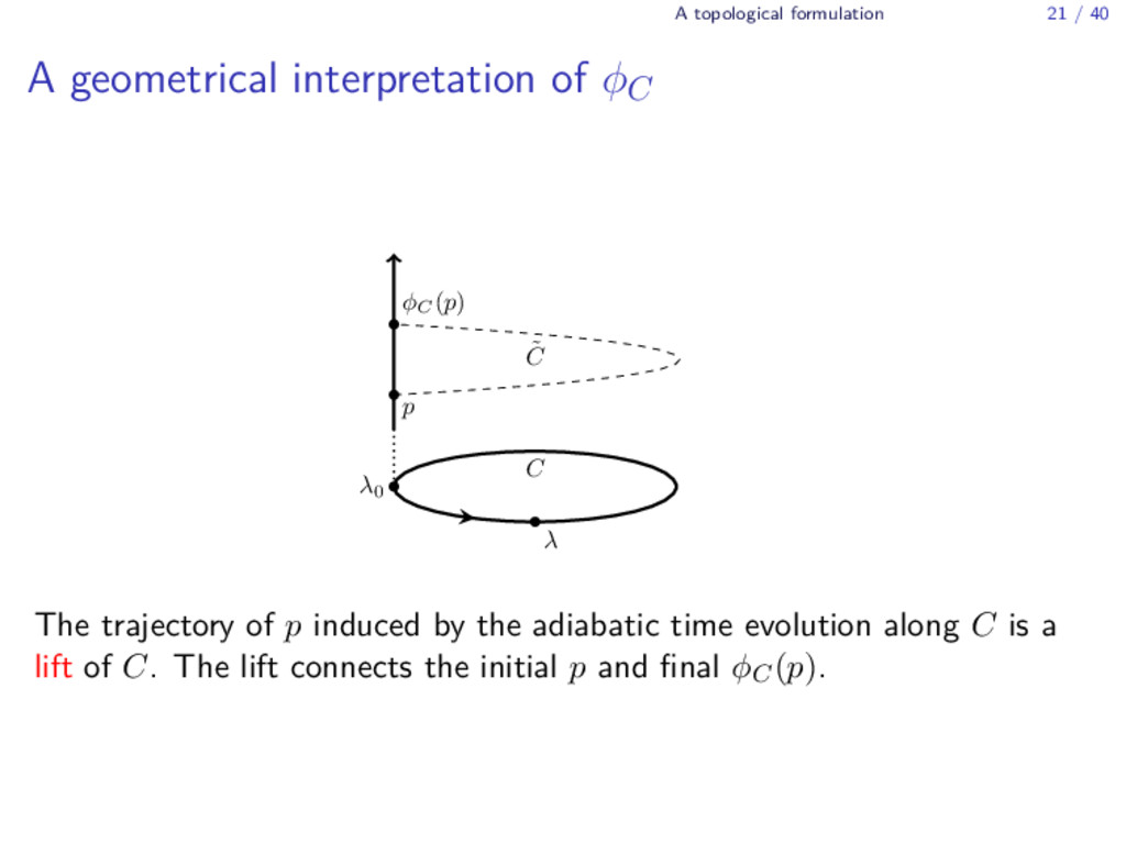
its mapping ϕC(p) The ordered eigenprojectors p ≡ ( ˆ P1, ˆ P2,...) where Pj is j-th eigenprojector. ϕC describes the change of p induced by C: ϕC( ˆ P1, ˆ P2) = { ( ˆ P1, ˆ P2) if C is trivial ( ˆ P2, ˆ P1) if C interchanges 1 and 2
ϕC p φC (p) C λ0 λ ˜ C The trajectory of p induced by the adiabatic time evolution along C is a lift of C. The lift connects the initial p and final ϕC(p).
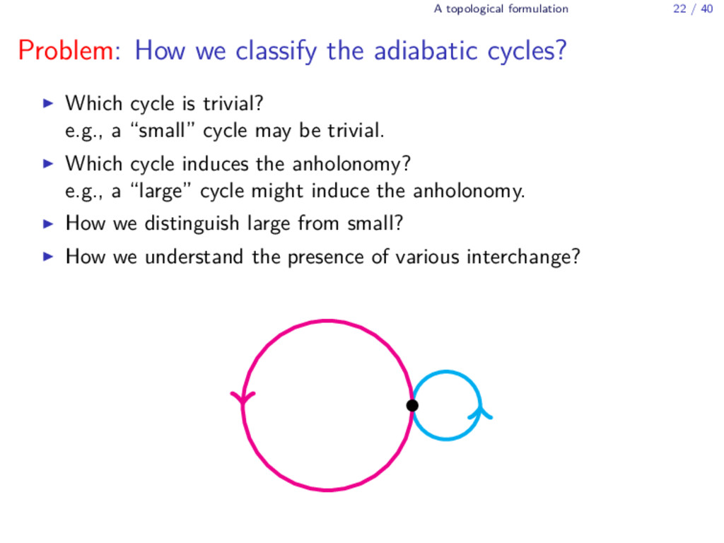
the adiabatic cycles? ▶ Which cycle is trivial? e.g., a “small” cycle may be trivial. ▶ Which cycle induces the anholonomy? e.g., a “large” cycle might induce the anholonomy. ▶ How we distinguish large from small? ▶ How we understand the presence of various interchange?
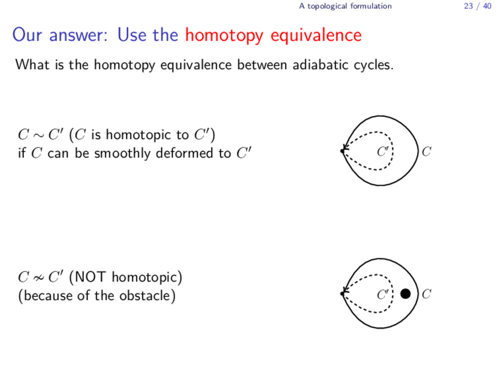
homotopy equivalence What is the homotopy equivalence between adiabatic cycles. C ∼ C′ (C is homotopic to C′) if C can be smoothly deformed to C′ C C C ≁ C′ (NOT homotopic) (because of the obstacle) C C
cycles in M The equivalent class of cycles for C: [C] ≡ { C′ C′ is a cycle in M, and, C′ ∼ C } The first fundamental group of M: π1(M) ≡ { [C] C is a cycle in M }
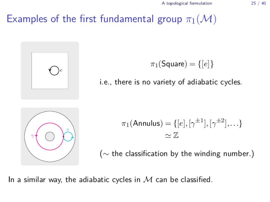
fundamental group π1(M) e π1(Square) = {[e]} i.e., there is no variety of adiabatic cycles. e γ π1(Annulus) = {[e],[γ±1],[γ±2],...} ≃ Z (∼ the classification by the winding number.) In a similar way, the adiabatic cycles in M can be classified.
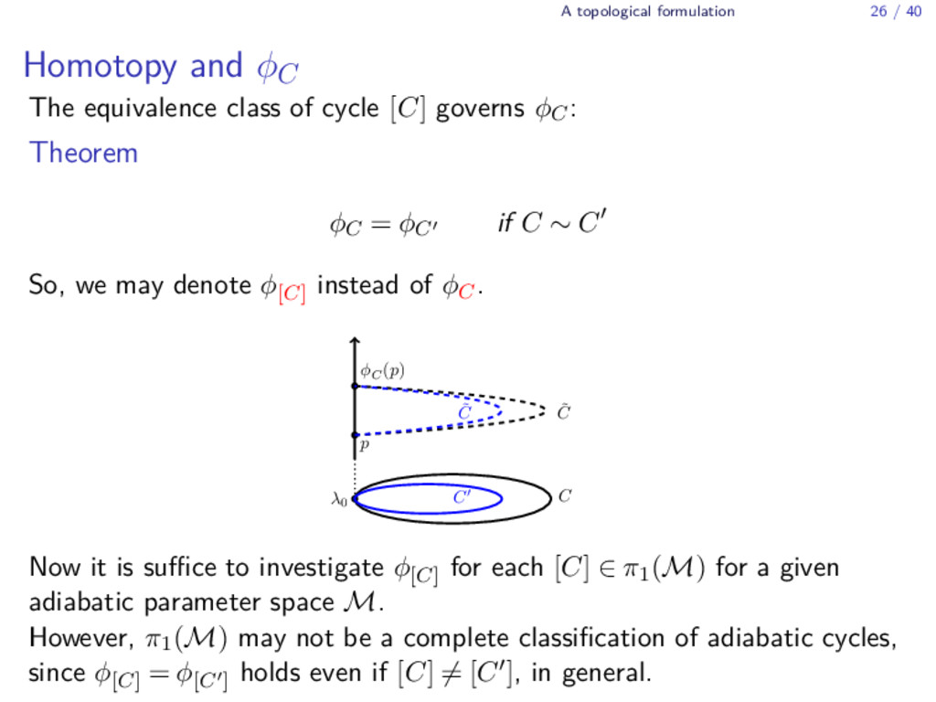
equivalence class of cycle [C] governs ϕC: Theorem ϕC = ϕC′ if C ∼ C′ So, we may denote ϕ[C] instead of ϕC. p φC (p) C λ0 C ˜ C ˜ C Now it is suffice to investigate ϕ[C] for each [C] ∈ π1(M) for a given adiabatic parameter space M. However, π1(M) may not be a complete classification of adiabatic cycles, since ϕ[C] = ϕ[C′] holds even if [C] ̸= [C′], in general.
ϕ[C] Under a certain condition, π1(M) offers a complete classification of the adiabatic cycles. Theorem ϕ[C] ̸= ϕ[C′] if [C] ̸= [C′] i.e., { ϕ[C] } [C]∈π1(M) ≃ π1(M), when the space of ( ˆ P1, ˆ P2,...) is “simple”.
1. Let M denote the adiabatic parameter space. 2. P consists of ordered eigenprojectors p = (P0, P1, ...). 3. ϕ[C] (the permutation of eigenspaces induced by C) and π1(M) has 1:1 correspondence, i.e. {ϕ[C] }[C]∈π1(M) ≃ π1(M), when P is “simple”. Hence the adiabatic cycles are completely classified by the homotopy equivalence, and it is suffice to examine ϕ[C] for each [C] ∈ π1(M). On the other hand, the analysis may strongly depends on model, as π1(M) may strongly depends on M.
space Let us introduce the set of eigenprojectors, where the order of the projectors is disregarded: b ≡ { ˆ P1, ˆ P2,...} (cf. p = ( ˆ P1, ˆ P2,...)) Let us denote b-space by B, which is a canonical adiabatic parameter space.
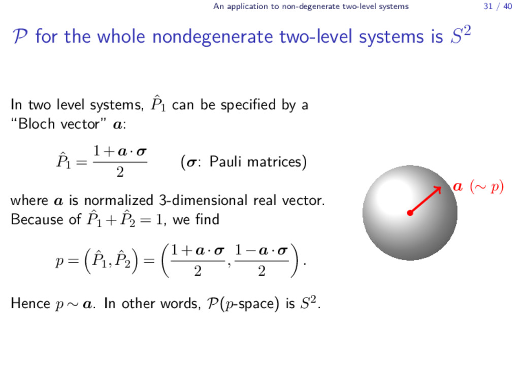
for the whole nondegenerate two-level systems is S2 In two level systems, ˆ P1 can be specified by a “Bloch vector” a: ˆ P1 = 1+a·σ 2 (σ: Pauli matrices) where a is normalized 3-dimensional real vector. Because of ˆ P1 + ˆ P2 = 1, we find p = ( ˆ P1, ˆ P2 ) = ( 1+a·σ 2 , 1−a·σ 2 ) . Hence p ∼ a. In other words, P(p-space) is S2. a (∼ p)
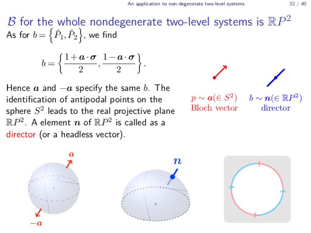
for the whole nondegenerate two-level systems is RP2 As for b = { ˆ P1, ˆ P2 } , we find b = { 1+a·σ 2 , 1−a·σ 2 } . Hence a and −a specify the same b. The identification of antipodal points on the sphere S2 leads to the real projective plane RP2. A element n of RP2 is called as a director (or a headless vector). p ∼ a(∈ S2) Bloch vector b ∼ n(∈ RP2) director a −a n
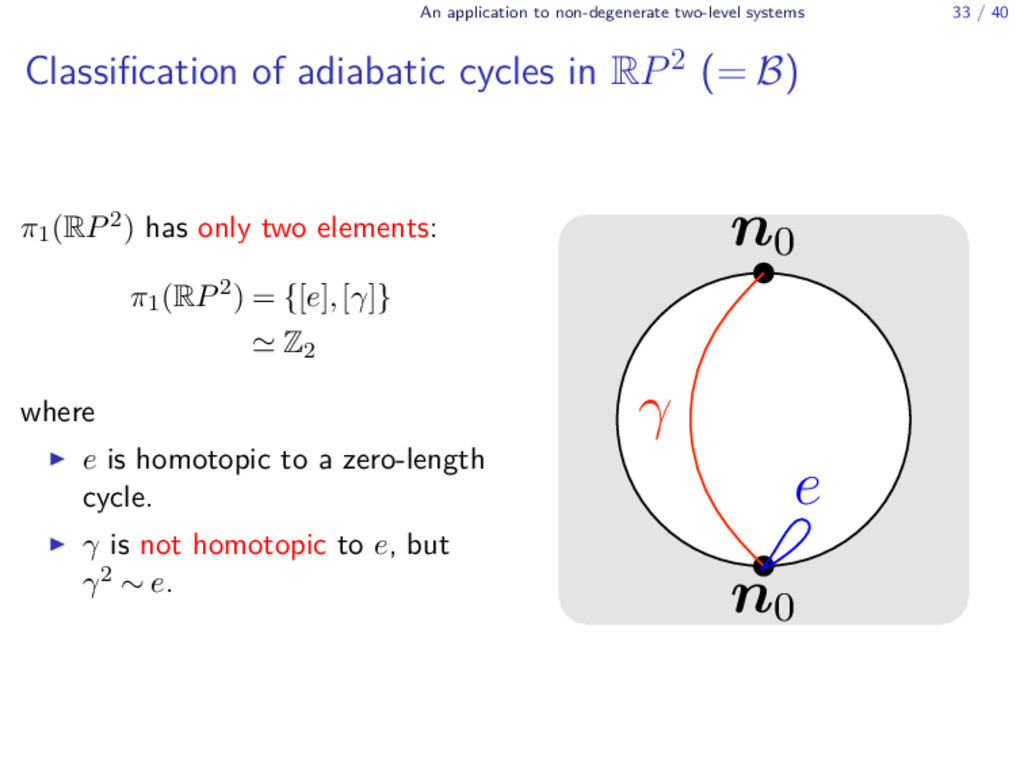
of adiabatic cycles in RP2 (= B) π1(RP2) has only two elements: π1(RP2) = {[e],[γ]} ≃ Z2 where ▶ e is homotopic to a zero-length cycle. ▶ γ is not homotopic to e, but γ2 ∼ e. n0 n0 γ e
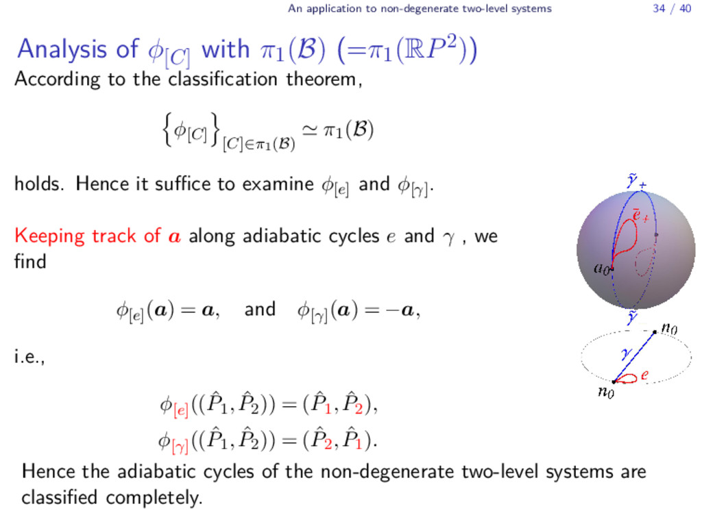
of ϕ[C] with π1(B) (=π1(RP2)) According to the classification theorem, { ϕ[C] } [C]∈π1(B) ≃ π1(B) holds. Hence it suffice to examine ϕ[e] and ϕ[γ] . Keeping track of a along adiabatic cycles e and γ , we find ϕ[e] (a) = a, and ϕ[γ] (a) = −a, i.e., ϕ[e] (( ˆ P1, ˆ P2)) = ( ˆ P1, ˆ P2), ϕ[γ] (( ˆ P1, ˆ P2)) = ( ˆ P2, ˆ P1). Hence the adiabatic cycles of the non-degenerate two-level systems are classified completely.
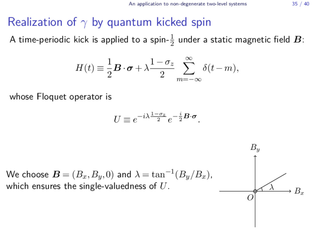
of γ by quantum kicked spin A time-periodic kick is applied to a spin-1 2 under a static magnetic field B: H(t) ≡ 1 2 B ·σ +λ 1−σz 2 ∞ ∑ m=−∞ δ(t−m), whose Floquet operator is U ≡ e−iλ 1−σz 2 e− i 2 B·σ. We choose B = (Bx,By,0) and λ = tan−1(By/Bx), which ensures the single-valuedness of U. Bx By O λ
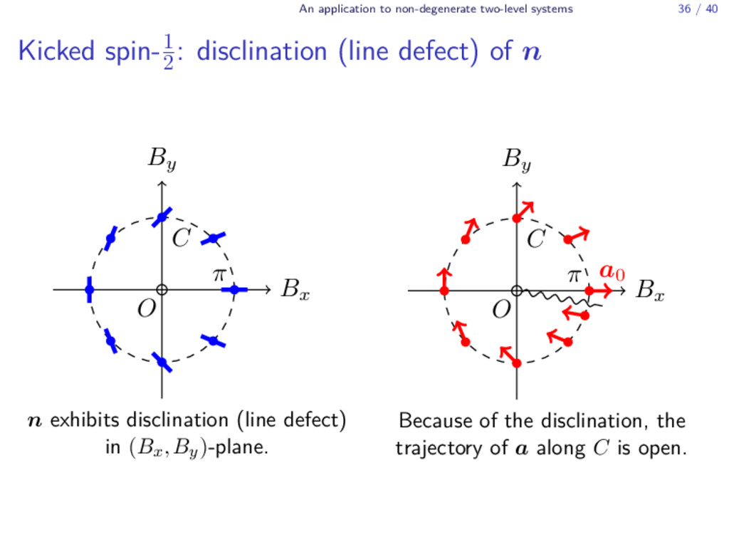
spin-1 2 : disclination (line defect) of n Bx By O π C n exhibits disclination (line defect) in (Bx,By)-plane. Bx By O C π a0 Because of the disclination, the trajectory of a along C is open.
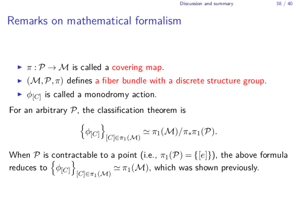
▶ π : P → M is called a covering map. ▶ (M,P,π) defines a fiber bundle with a discrete structure group. ▶ ϕ[C] is called a monodromy action. For an arbitrary P, the classification theorem is { ϕ[C] } [C]∈π1(M) ≃ π1(M)/π∗π1(P). When P is contractable to a point (i.e., π1(P) = {[e]}), the above formula reduces to { ϕ[C] } [C]∈π1(M) ≃ π1(M), which was shown previously.
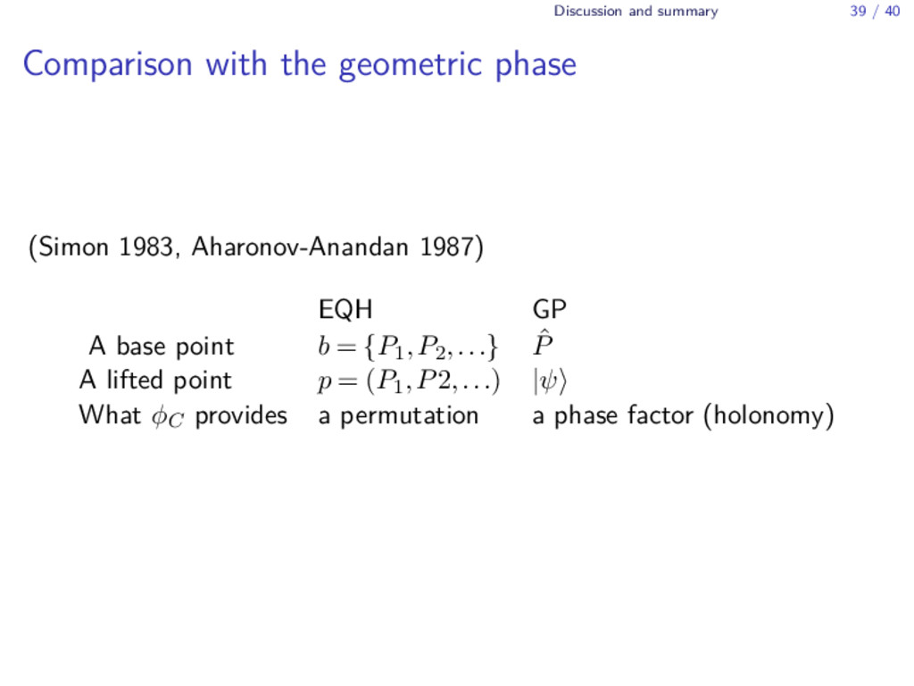
phase (Simon 1983, Aharonov-Anandan 1987) EQH GP A base point b = {P1,P2,...} ˆ P A lifted point p = (P1,P2,...) |ψ⟩ What ϕC provides a permutation a phase factor (holonomy)
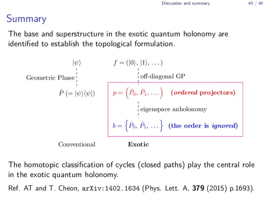
superstructure in the exotic quantum holonomy are identified to establish the topological formulation. |ψ f = (|0 , |1 , . . . ) ˆ P (= |ψ ψ|) p = ˆ P0 , ˆ P1 , . . . (ordered projectors) b = ˆ P0 , ˆ P1 , . . . (the order is ignored) Conventional Exotic Geometric Phase off-diagonal GP eigenspace anholonomy The homotopic classification of cycles (closed paths) play the central role in the exotic quantum holonomy. Ref. AT and T. Cheon, arXiv:1402.1634 (Phys. Lett. A, 379 (2015) p.1693).