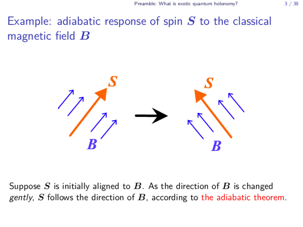
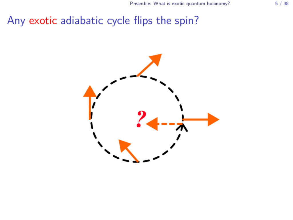
adiabatic response of spin S to the classical magnetic field B Suppose S is initially aligned to B. As the direction of B is changed gently, S follows the direction of B, according to the adiabatic theorem.
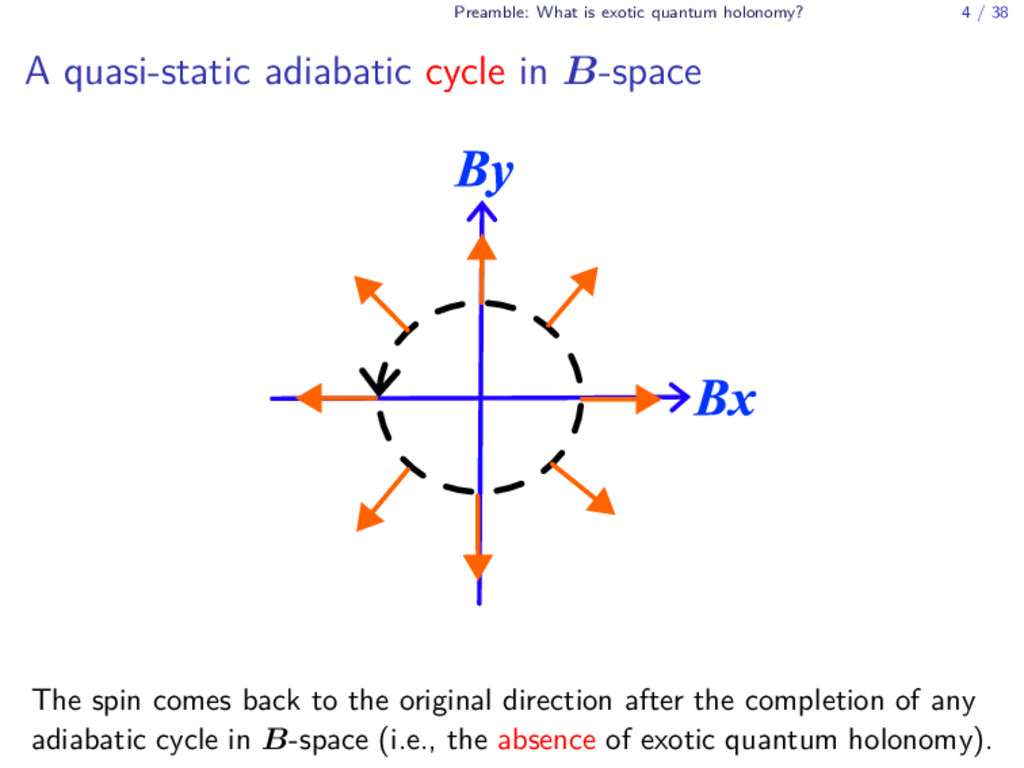
quasi-static adiabatic cycle in B-space The spin comes back to the original direction after the completion of any adiabatic cycle in B-space (i.e., the absence of exotic quantum holonomy).
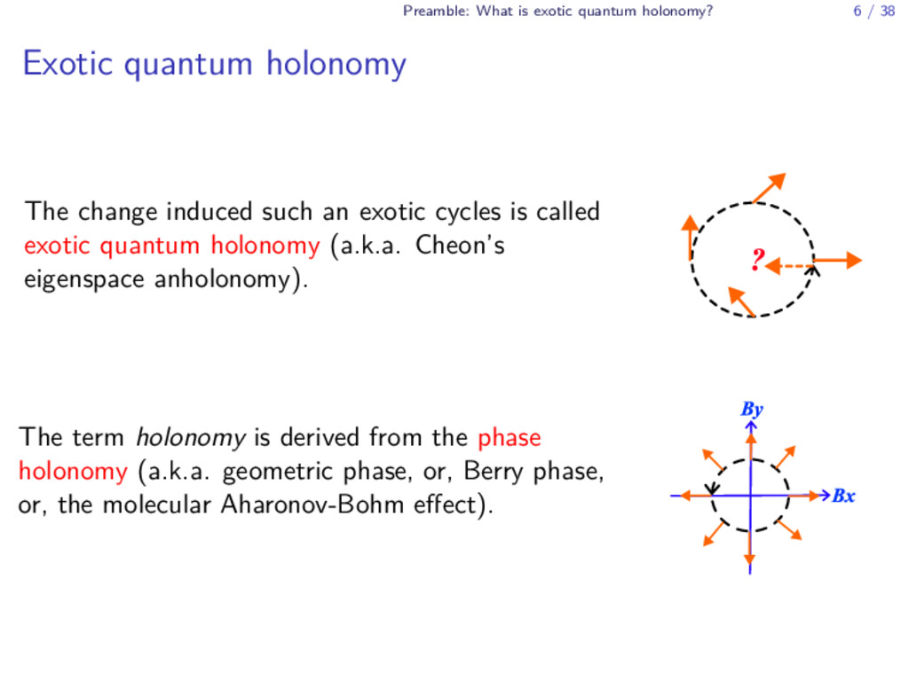
quantum holonomy The change induced such an exotic cycles is called exotic quantum holonomy (a.k.a. Cheon’s eigenspace anholonomy). The term holonomy is derived from the phase holonomy (a.k.a. geometric phase, or, Berry phase, or, the molecular Aharonov-Bohm effect).
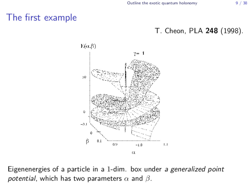
1. Provide an outline of the exotic quantum holonomy 2. Explain a topological formulation of the exotic quantum holonomy Ref. AT and T. Cheon, arXiv:1402.1634 (Phys. Lett. A, 379 (2015) p.1693) and references therein.
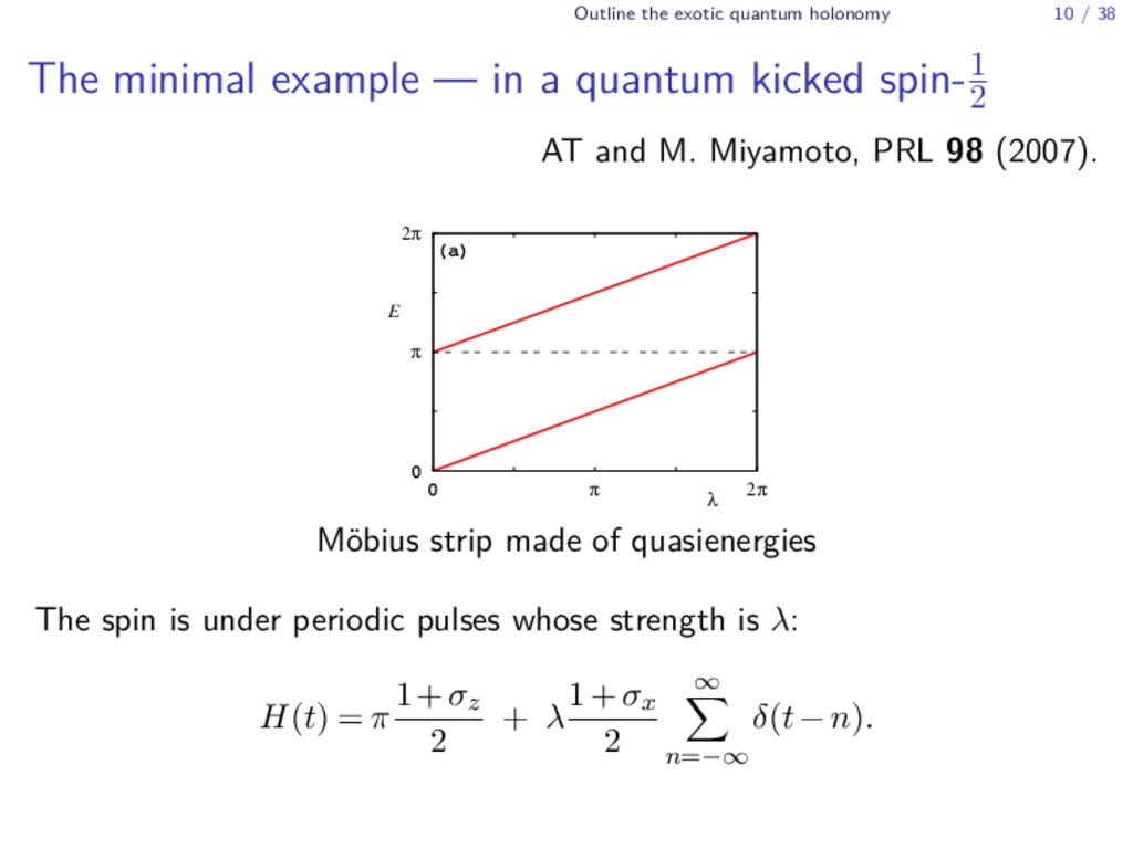
example — in a quantum kicked spin-1 2 AT and M. Miyamoto, PRL 98 (2007). 2π π 0 2π π 0 (a) λ E M¨ obius strip made of quasienergies The spin is under periodic pulses whose strength is λ: H(t) = π 1+σz 2 + λ 1+σx 2 ∞ ∑ n=−∞ δ(t−n).
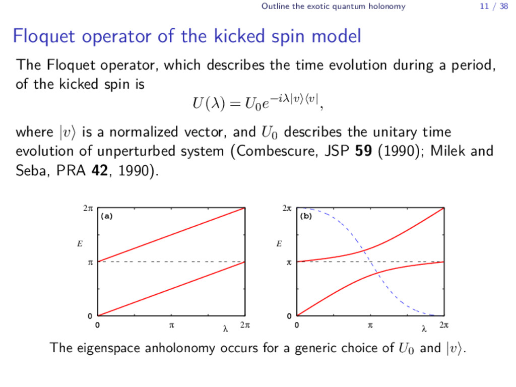
of the kicked spin model The Floquet operator, which describes the time evolution during a period, of the kicked spin is U(λ) = U0e−iλ|v⟩⟨v|, where |v⟩ is a normalized vector, and U0 describes the unitary time evolution of unperturbed system (Combescure, JSP 59 (1990); Milek and Seba, PRA 42, 1990). 2π π 0 2π π 0 (a) λ E 2π π 0 2π π 0 (b) λ E The eigenspace anholonomy occurs for a generic choice of U0 and |v⟩.
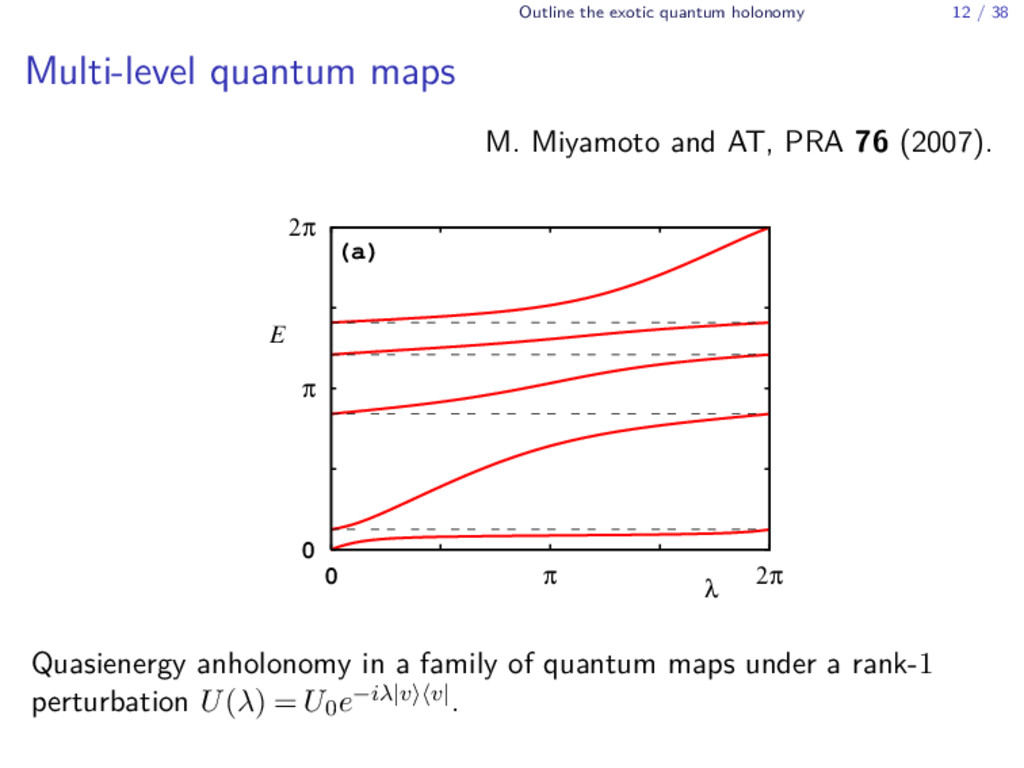
maps M. Miyamoto and AT, PRA 76 (2007). 2π π 0 2π π 0 (a) λ E Quasienergy anholonomy in a family of quantum maps under a rank-1 perturbation U(λ) = U0e−iλ|v⟩⟨v|.
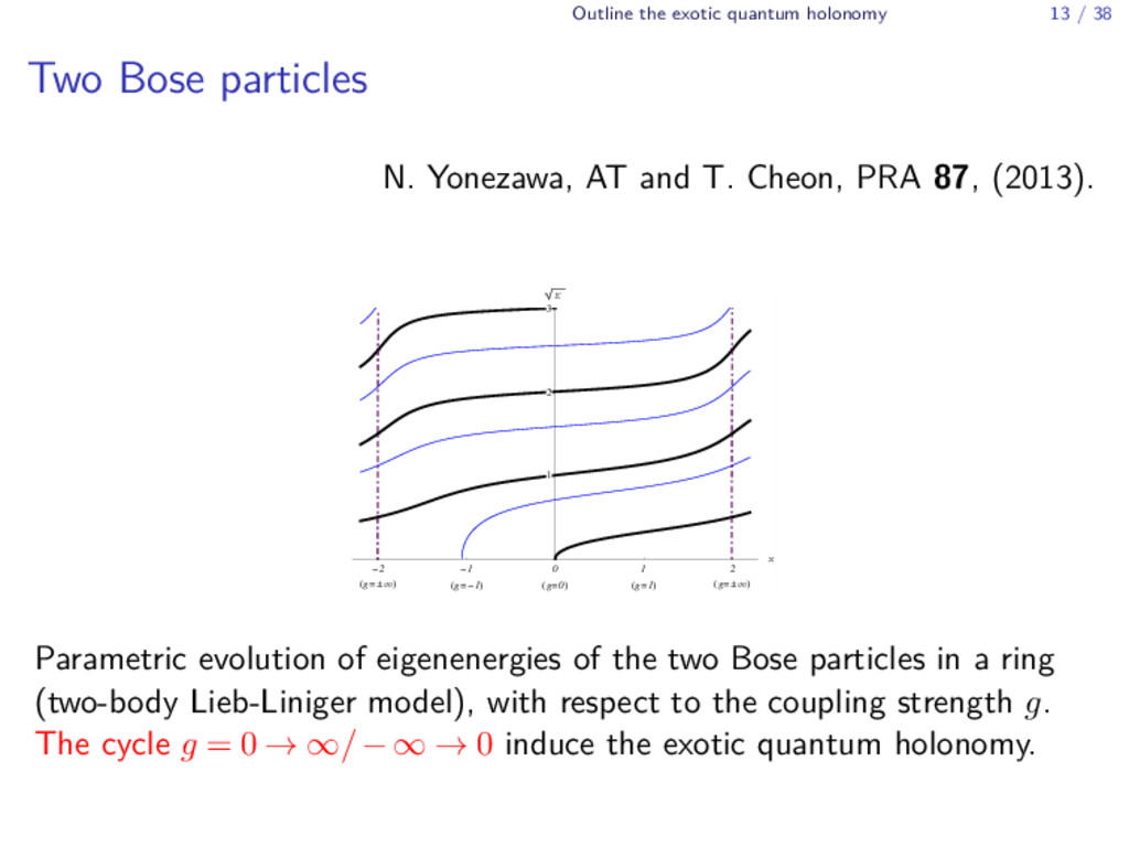
particles N. Yonezawa, AT and T. Cheon, PRA 87, (2013). 2 g 1 g 1 0 g 0 1 g 1 2 g x 1 2 3 E Parametric evolution of eigenenergies of the two Bose particles in a ring (two-body Lieb-Liniger model), with respect to the coupling strength g. The cycle g = 0 → ∞/−∞ → 0 induce the exotic quantum holonomy.
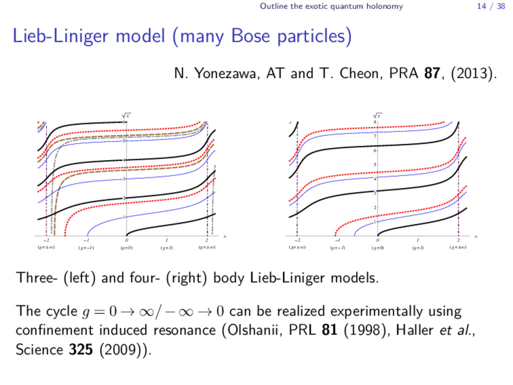
(many Bose particles) N. Yonezawa, AT and T. Cheon, PRA 87, (2013). 2 g 1 g 1 0 g 0 1 g 1 2 g x 1 2 3 4 5 6 E 2 g 1 g 1 0 g 0 1 g 1 2 g x 1 2 3 4 5 6 7 8 E Three- (left) and four- (right) body Lieb-Liniger models. The cycle g = 0 → ∞/−∞ → 0 can be realized experimentally using confinement induced resonance (Olshanii, PRL 81 (1998), Haller et al., Science 325 (2009)).
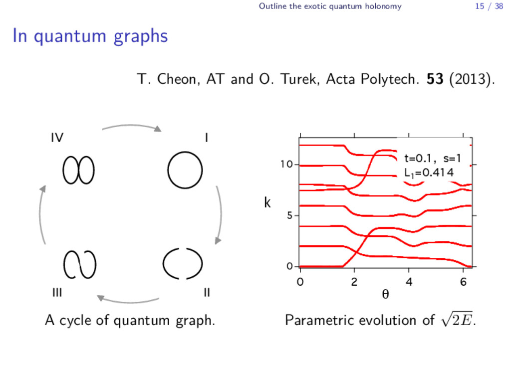
graphs T. Cheon, AT and O. Turek, Acta Polytech. 53 (2013). II V I II III IV A cycle of quantum graph. 10 5 0 k 6 4 2 0 θ t=0.1, s=1 L1 =0.414 Parametric evolution of √ 2E.
▶ Quantum graphs/Generalized contact potentials (I. Tsutsui, T. F¨ ulop and T. Cheon 2000; I. Tsutsui, T. F¨ ulop and T. Cheon 2001; S. Ohya, Ann. Phys. 331 (2013); S. Ohya, Ann. Phys. 351 (2014)) ▶ Non-Abelian extension (T. Cheon and AT 2009) ▶ Nonadiabatic example in time-dependent Aharonov-Bohm ring (AT and T. Cheon 2010) ▶ Accelerating adiabatic quantum computation (AT and K. Nemoto 2010) ▶ Hierarchical many-qubit systems (AT, S. W. Kim and T. Cheon 2011; AT, T. Cheon and S. W. Kim 2012) ▶ Autonomous Hamiltonians (T. Cheon, AT and S. W. Kim, 2009) ▶ Another good example?
▶ Generalized Fujikawa formalism (T. Cheon and AT 2009; AT and T. Cheon 2009) . . . the eigenspace anholonomy and the off-diagonal geometric phase factors (Manini and Pistolesi, PRL 85 (2000)) are entangled ▶ Exotic quantum holonomy as an encirclement of non-Hermitian degeneracy points by Hermitian Hamiltonian/unitary Floquet operators. (S. W. Kim, T. Cheon and AT 2010; AT, N. Yonezawa and T. Cheon 2013; AT, S. W. Kim and T. Cheon 2014) . . . requires an analytic continuation of parameters ▶ Abelian gerbes in adiabatic Floquet theory (Viennot, JPA 42 (2009)) . . . applicable only to periodically driven systems ▶ Another good theory? . . . the main subject of the next section
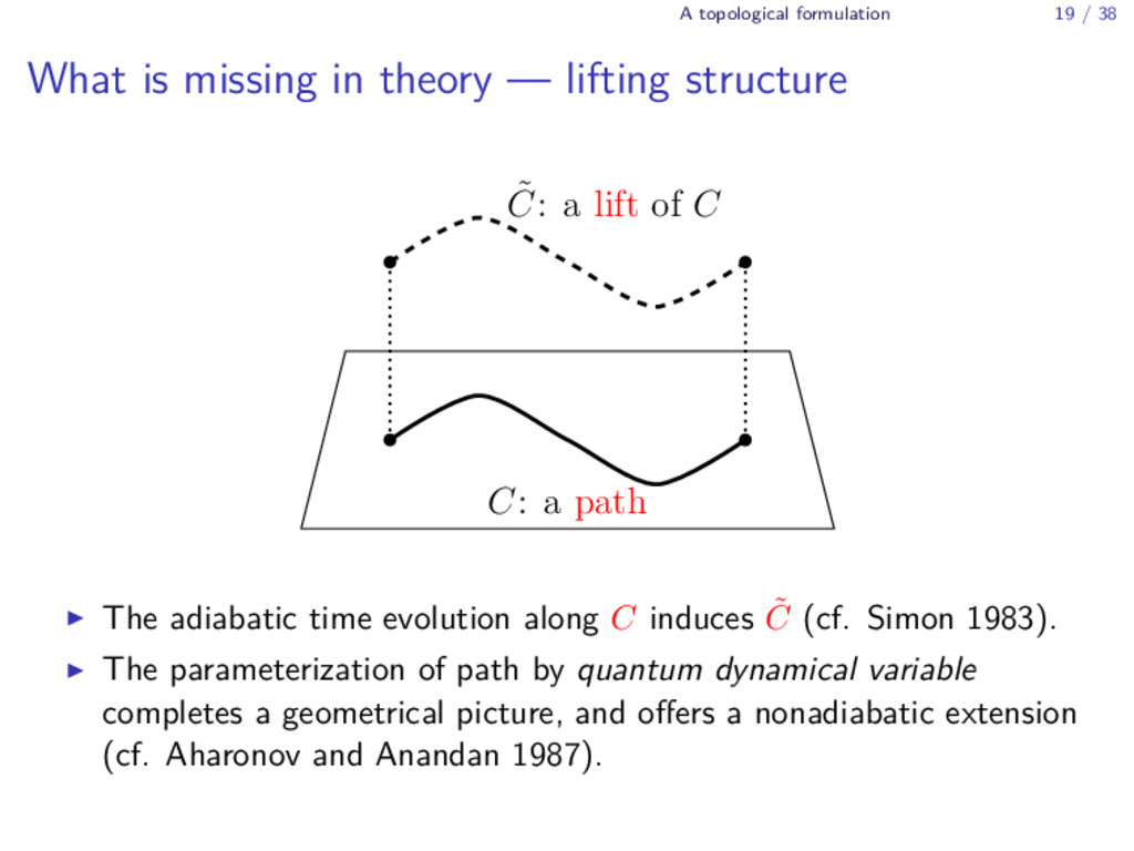
theory — lifting structure C: a path ˜ C: a lift of C ▶ The adiabatic time evolution along C induces ˜ C (cf. Simon 1983). ▶ The parameterization of path by quantum dynamical variable completes a geometrical picture, and offers a nonadiabatic extension (cf. Aharonov and Anandan 1987).
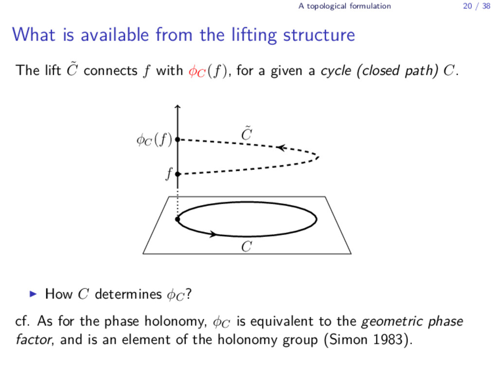
the lifting structure The lift ˜ C connects f with ϕC(f), for a given a cycle (closed path) C. f φC (f) C ˜ C ▶ How C determines ϕC? cf. As for the phase holonomy, ϕC is equivalent to the geometric phase factor, and is an element of the holonomy group (Simon 1983).
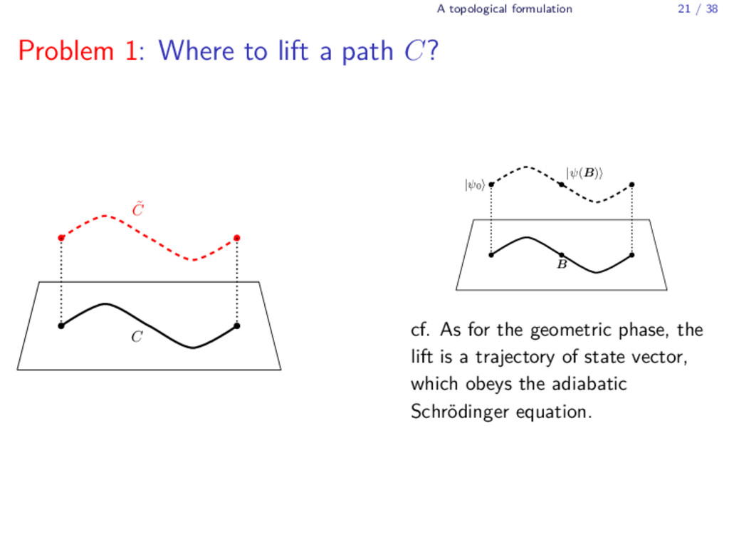
lift a path C? C ˜ C B |ψ0 |ψ(B) cf. As for the geometric phase, the lift is a trajectory of state vector, which obeys the adiabatic Schr¨ odinger equation.
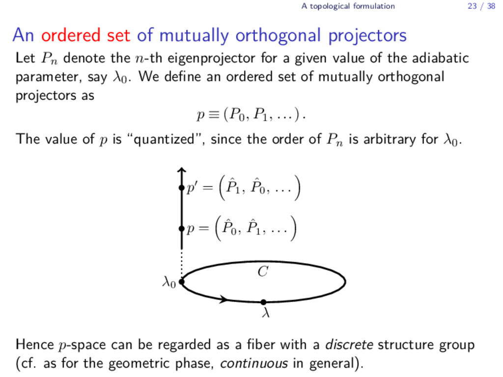
mutually orthogonal projectors Let Pn denote the n-th eigenprojector for a given value of the adiabatic parameter, say λ0. We define an ordered set of mutually orthogonal projectors as p ≡ (P0, P1, ...). The value of p is “quantized”, since the order of Pn is arbitrary for λ0. p = ˆ P0 , ˆ P1 , . . . p = ˆ P1 , ˆ P0 , . . . C λ0 λ Hence p-space can be regarded as a fiber with a discrete structure group (cf. as for the geometric phase, continuous in general).
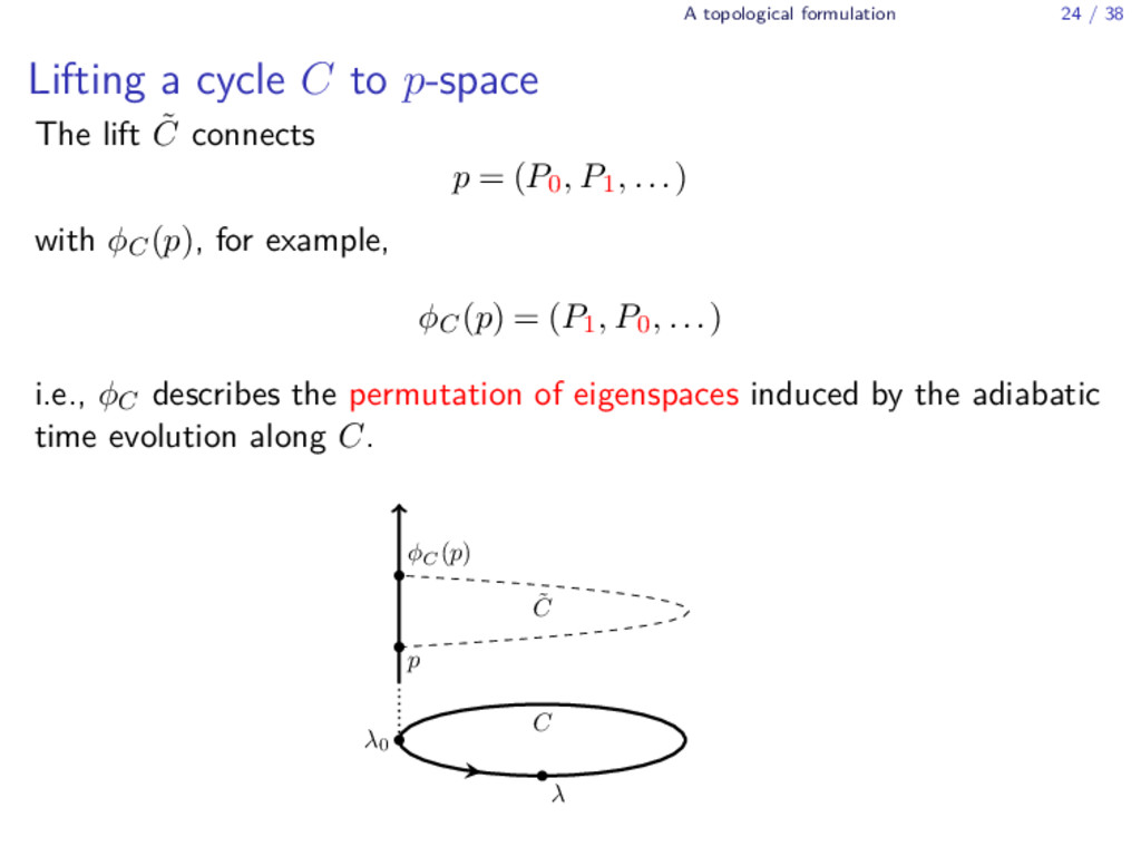
to p-space The lift ˜ C connects p = (P0, P1, ...) with ϕC(p), for example, ϕC(p) = (P1, P0, ...) i.e., ϕC describes the permutation of eigenspaces induced by the adiabatic time evolution along C. p φC (p) C λ0 λ ˜ C
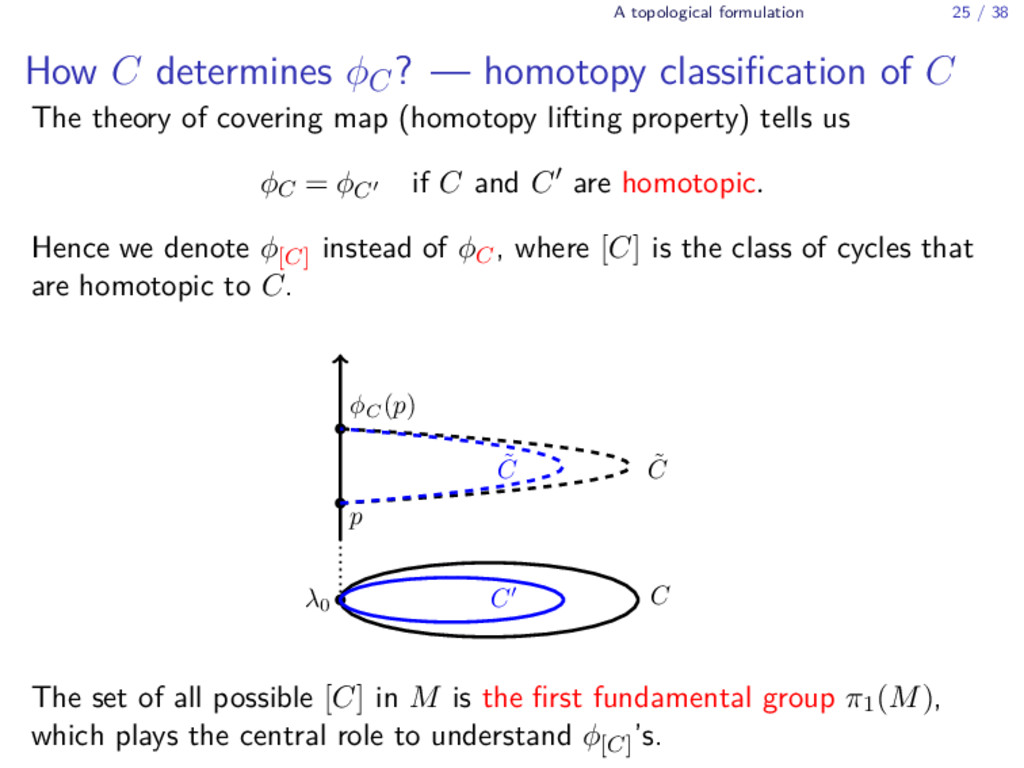
— homotopy classification of C The theory of covering map (homotopy lifting property) tells us ϕC = ϕC′ if C and C′ are homotopic. Hence we denote ϕ[C] instead of ϕC, where [C] is the class of cycles that are homotopic to C. p φC (p) C λ0 C ˜ C ˜ C The set of all possible [C] in M is the first fundamental group π1(M), which plays the central role to understand ϕ[C] ’s.
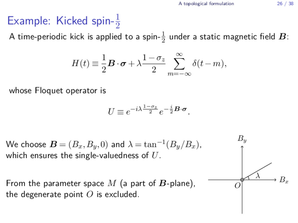
A time-periodic kick is applied to a spin-1 2 under a static magnetic field B: H(t) ≡ 1 2 B ·σ +λ 1−σz 2 ∞ ∑ m=−∞ δ(t−m), whose Floquet operator is U ≡ e−iλ 1−σz 2 e− i 2 B·σ. We choose B = (Bx,By,0) and λ = tan−1(By/Bx), which ensures the single-valuedness of U. From the parameter space M (a part of B-plane), the degenerate point O is excluded. Bx By O λ
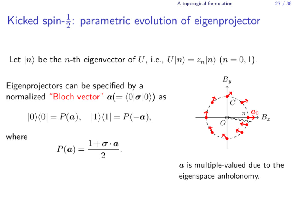
parametric evolution of eigenprojector Let |n⟩ be the n-th eigenvector of U, i.e., U|n⟩ = zn|n⟩ (n = 0,1). Eigenprojectors can be specified by a normalized “Bloch vector” a(= ⟨0|σ|0⟩) as |0⟩⟨0| = P(a), |1⟩⟨1| = P(−a), where P(a) = 1+σ ·a 2 . Bx By O C π a0 a is multiple-valued due to the eigenspace anholonomy.
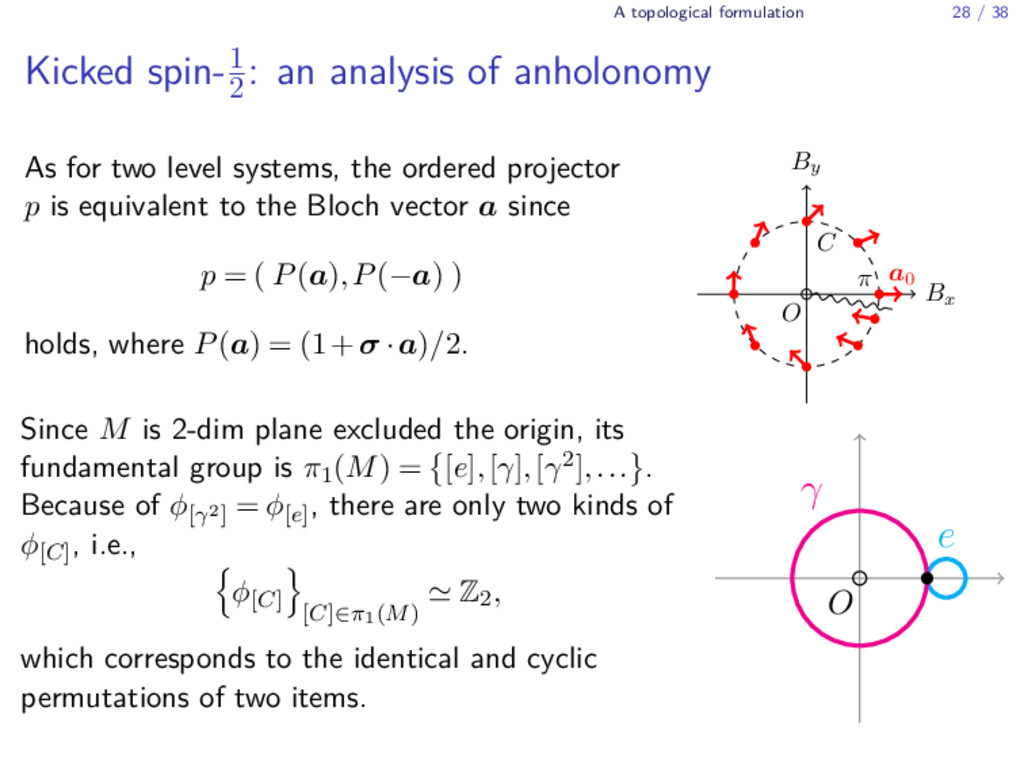
an analysis of anholonomy As for two level systems, the ordered projector p is equivalent to the Bloch vector a since p = ( P(a),P(−a) ) holds, where P(a) = (1+σ ·a)/2. Bx By O C π a0 Since M is 2-dim plane excluded the origin, its fundamental group is π1(M) = { [e],[γ],[γ2],... } . Because of ϕ[γ2] = ϕ[e] , there are only two kinds of ϕ[C] , i.e., { ϕ[C] } [C]∈π1(M) ≃ Z2, which corresponds to the identical and cyclic permutations of two items. O e γ
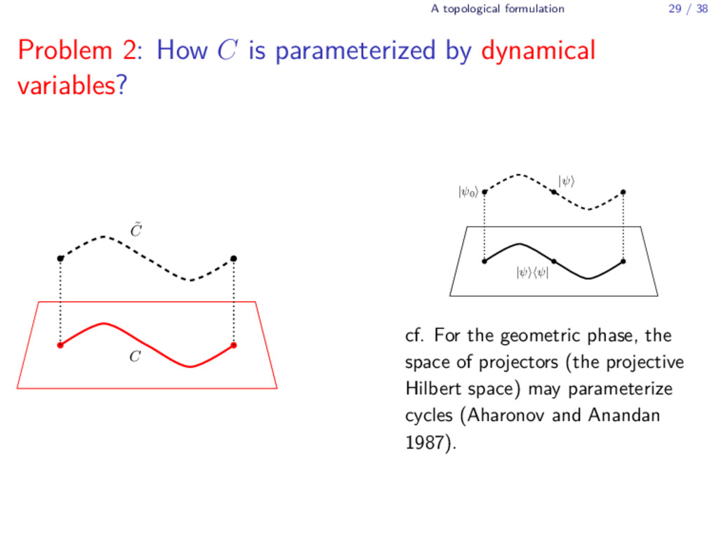
is parameterized by dynamical variables? C ˜ C |ψ ψ| |ψ0 |ψ cf. For the geometric phase, the space of projectors (the projective Hilbert space) may parameterize cycles (Aharonov and Anandan 1987).
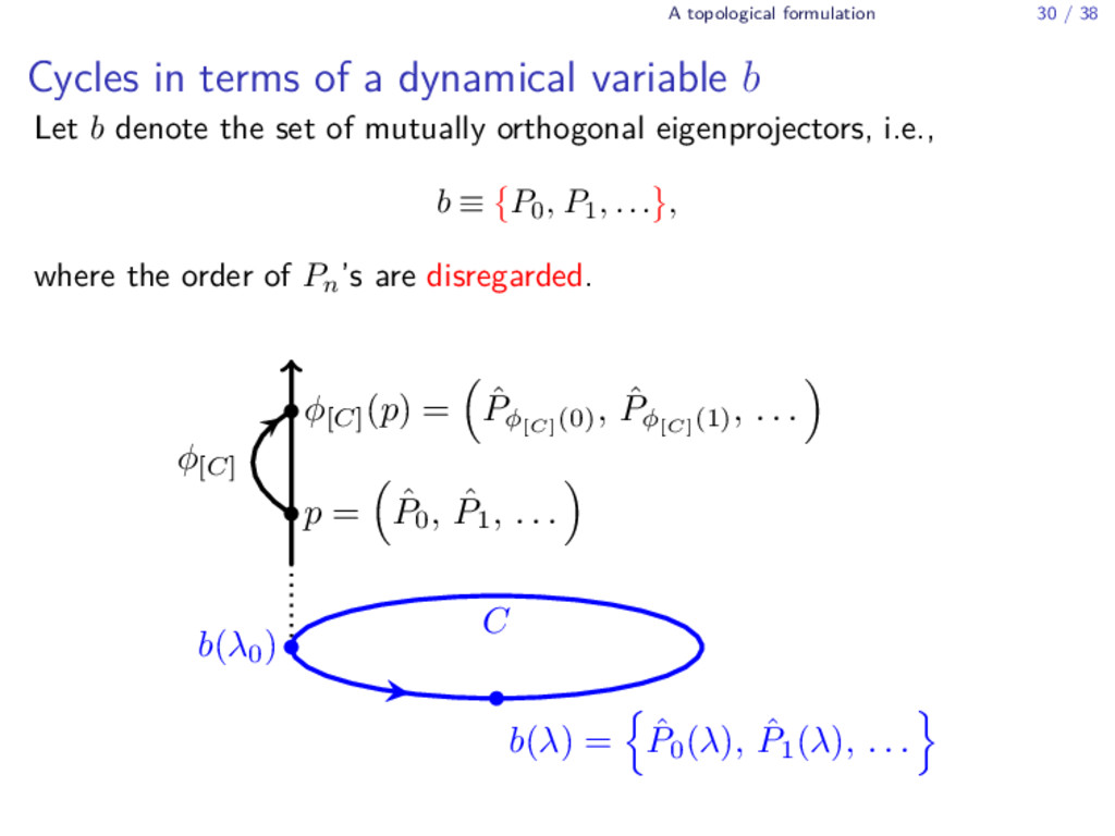
a dynamical variable b Let b denote the set of mutually orthogonal eigenprojectors, i.e., b ≡ { P0, P1, ... } , where the order of Pn’s are disregarded. p = ˆ P0 , ˆ P1 , . . . φ[C] (p) = ˆ Pφ[C] (0) , ˆ Pφ[C] (1) , . . . φ[C] C b(λ0 ) b(λ) = ˆ P0 (λ), ˆ P1 (λ), . . .
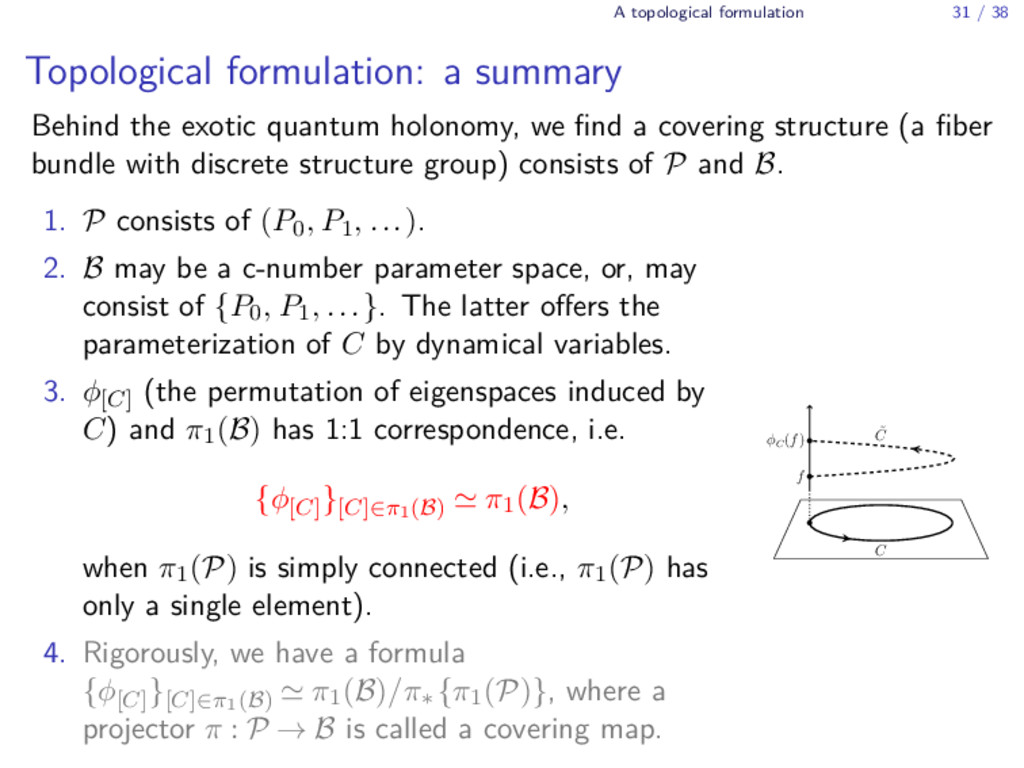
Behind the exotic quantum holonomy, we find a covering structure (a fiber bundle with discrete structure group) consists of P and B. 1. P consists of (P0, P1, ...). 2. B may be a c-number parameter space, or, may consist of {P0, P1, ...}. The latter offers the parameterization of C by dynamical variables. 3. ϕ[C] (the permutation of eigenspaces induced by C) and π1(B) has 1:1 correspondence, i.e. {ϕ[C] }[C]∈π1(B) ≃ π1(B), when π1(P) is simply connected (i.e., π1(P) has only a single element). 4. Rigorously, we have a formula {ϕ[C] }[C]∈π1(B) ≃ π1(B)/π∗ {π1(P)}, where a projector π : P → B is called a covering map. f φC (f) C ˜ C
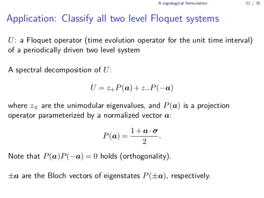
level Floquet systems U: a Floquet operator (time evolution operator for the unit time interval) of a periodically driven two level system A spectral decomposition of U: U = z+P(a)+z−P(−a) where z± are the unimodular eigenvalues, and P(a) is a projection operator parameterized by a normalized vector a: P(a) = 1+a·σ 2 . Note that P(a)P(−a) = 0 holds (orthogonality). ±a are the Bloch vectors of eigenstates P(±a), respectively.
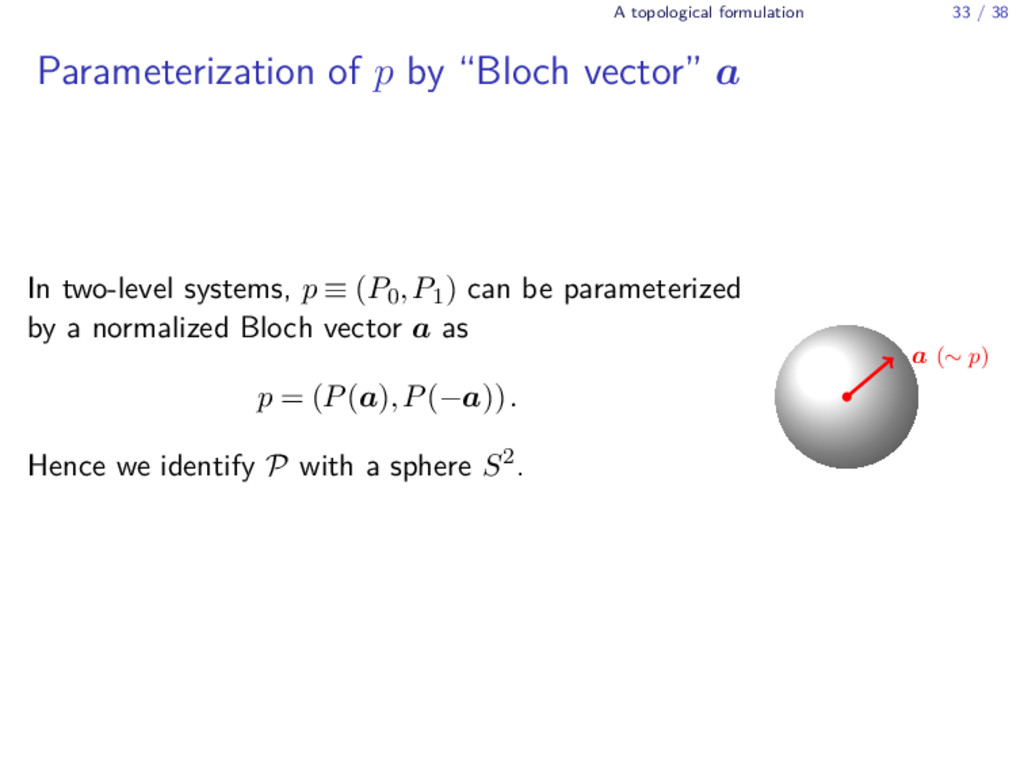
“Bloch vector” a In two-level systems, p ≡ (P0,P1) can be parameterized by a normalized Bloch vector a as p = (P(a),P(−a)). Hence we identify P with a sphere S2. a (∼ p)
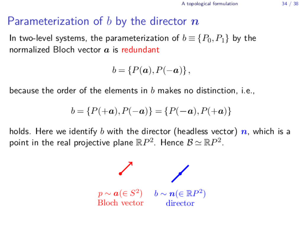
the director n In two-level systems, the parameterization of b ≡ {P0,P1} by the normalized Bloch vector a is redundant b = {P(a),P(−a)}, because the order of the elements in b makes no distinction, i.e., b = {P(+a),P(−a)} = {P(−a),P(+a)} holds. Here we identify b with the director (headless vector) n, which is a point in the real projective plane RP2. Hence B ≃ RP2. p ∼ a(∈ S2) Bloch vector b ∼ n(∈ RP2) director
group π1(B) For two level systems, because of π1(P) = 1 (∵ P ≃ S2), {ϕ[C] }[C]∈π1(B) ≃ π1(B) holds, i.e., π1(B) governs the eigenspace anholonomy (B = RP2). Each element of π1(RP2) = {[e], [γ]} has a 1 : 1 correspondence with the permutation σ of the eigenspaces. ▶ [e] ↔ the identical permutation (∼ the absence of the anholonomy) ▶ [γ] ↔ the cyclic permutation (∼ the presence the anholonomy) Hence {ϕ[C] }[C]∈π1(B) ≃ Z2 also holds here.
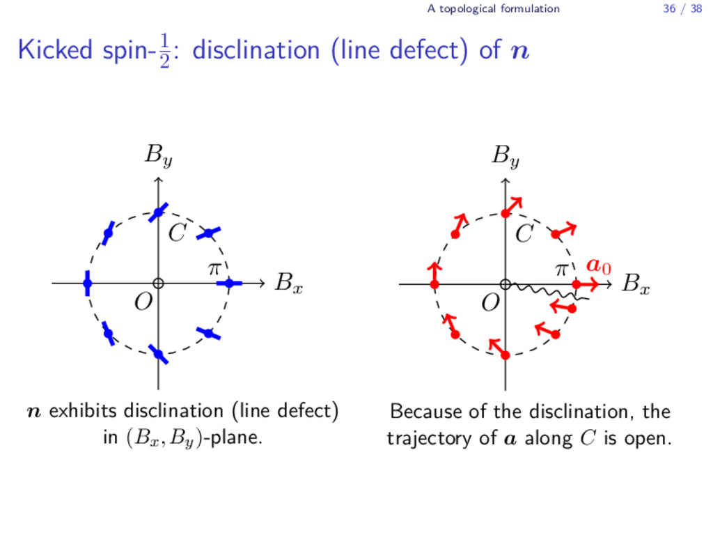
disclination (line defect) of n Bx By O π C n exhibits disclination (line defect) in (Bx,By)-plane. Bx By O C π a0 Because of the disclination, the trajectory of a along C is open.
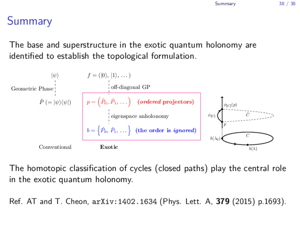
the exotic quantum holonomy are identified to establish the topological formulation. |ψ f = (|0 , |1 , . . . ) ˆ P (= |ψ ψ|) p = ˆ P0 , ˆ P1 , . . . (ordered projectors) b = ˆ P0 , ˆ P1 , . . . (the order is ignored) Conventional Exotic Geometric Phase off-diagonal GP eigenspace anholonomy p φ[C] (p) φ[C] C b(λ0 ) b(λ) ˜ C The homotopic classification of cycles (closed paths) play the central role in the exotic quantum holonomy. Ref. AT and T. Cheon, arXiv:1402.1634 (Phys. Lett. A, 379 (2015) p.1693).
![A topological formulation 35 / 38 ϕ[C] and the fundamental](https://files.speakerdeck.com/presentations/d646f174de8d4bd7a024b358356d11ae/slide_34.jpg)