Path topology dependence of adiabatic time evolution / 断熱的な時間発展の結果は経路のトポロジーで決まる

Presented at JPS September meeting (14pAF, 2016-09-14) / 日本物理学会 2016年秋季大会での口頭発表 (14pAF, 9月14日)

Transcript

1. 1 / 18 Path topology dependence of adiabatic time evolution ɹʢஅ೤తͳ࣌ؒൃలͷ݁Ռ͸ܦ࿏ͷτϙϩδʔͰܾ·Δʣ Atushi Tanaka (ాதಞ࢘), Taksu Cheon (શ୎थ)A Tokyo Metropolitan Univ. (ट౎େཧ޻), Kochi Univ. Tech. (ߴ஌޻Պେ)A 2016-09-14 Ref. arXiv:1512.06983 ೔ຊ෺ཧֶձ̎̌̍̒೥ळقେձʦ෺ੑʧۚ୔େֶʢ֯ؒΩϟϯύεʣ(2016-09-13/2016-09-16) 14pAF-1
2. 2 / 18 Outline Introduction Lifting adiabatic paths Classify adiabatic paths in terms of homotopy Summary
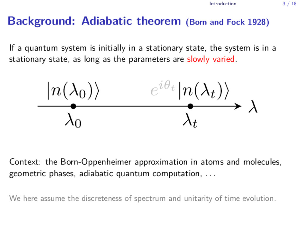
3. Introduction 3 / 18 Background: Adiabatic theorem (Born and Fock 1928) If a quantum system is initially in a stationary state, the system is in a stationary state, as long as the parameters are slowly varied. λ λ0 λt |n(λ0 ) eiθt |n(λt ) Context: the Born-Oppenheimer approximation in atoms and molecules, geometric phases, adiabatic quantum computation, . . . We here assume the discreteness of spectrum and unitarity of time evolution.
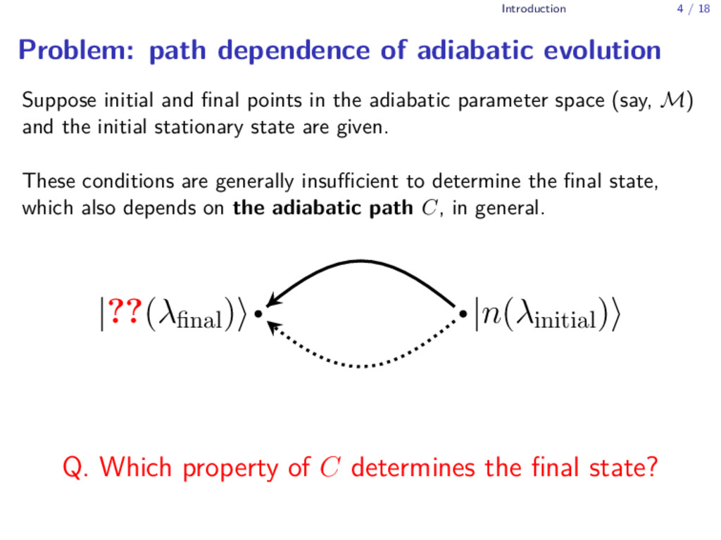
4. Introduction 4 / 18 Problem: path dependence of adiabatic evolution Suppose initial and final points in the adiabatic parameter space (say, M) and the initial stationary state are given. These conditions are generally insufficient to determine the final state, which also depends on the adiabatic path C, in general. |n(λinitial ) |??(λfinal ) Q. Which property of C determines the final state?
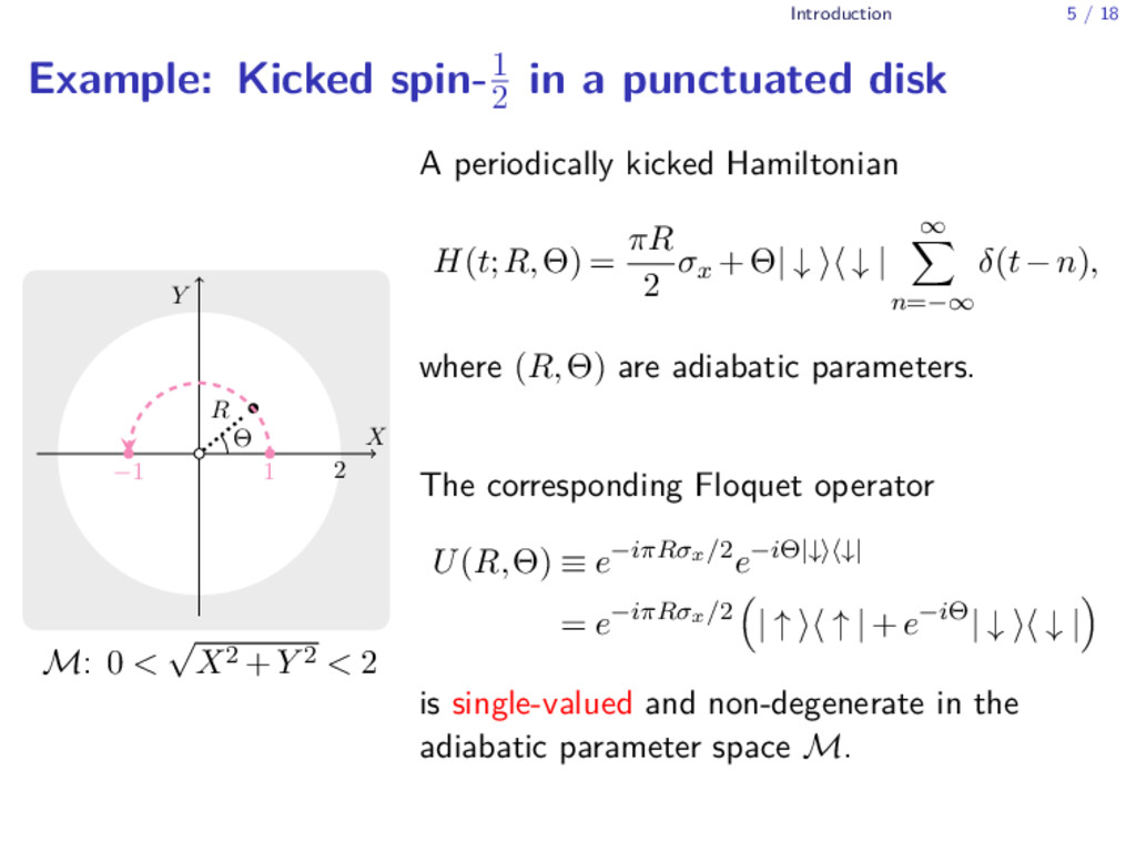
5. Introduction 5 / 18 Example: Kicked spin-1 2 in a punctuated disk O X Y 2 Θ R 1 −1 M: 0 < √ X2 +Y 2 < 2 A periodically kicked Hamiltonian H(t;R,Θ) = πR 2 σx +Θ| ↓ ⟩⟨ ↓ | ∞ ∑ n=−∞ δ(t−n), where (R,Θ) are adiabatic parameters. The corresponding Floquet operator U(R,Θ) ≡ e−iπRσx/2e−iΘ|↓⟩⟨↓| = e−iπRσx/2 ( | ↑ ⟩⟨ ↑ |+e−iΘ| ↓ ⟩⟨ ↓ | ) is single-valued and non-degenerate in the adiabatic parameter space M.
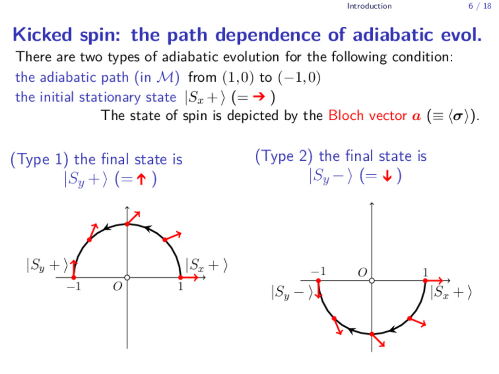
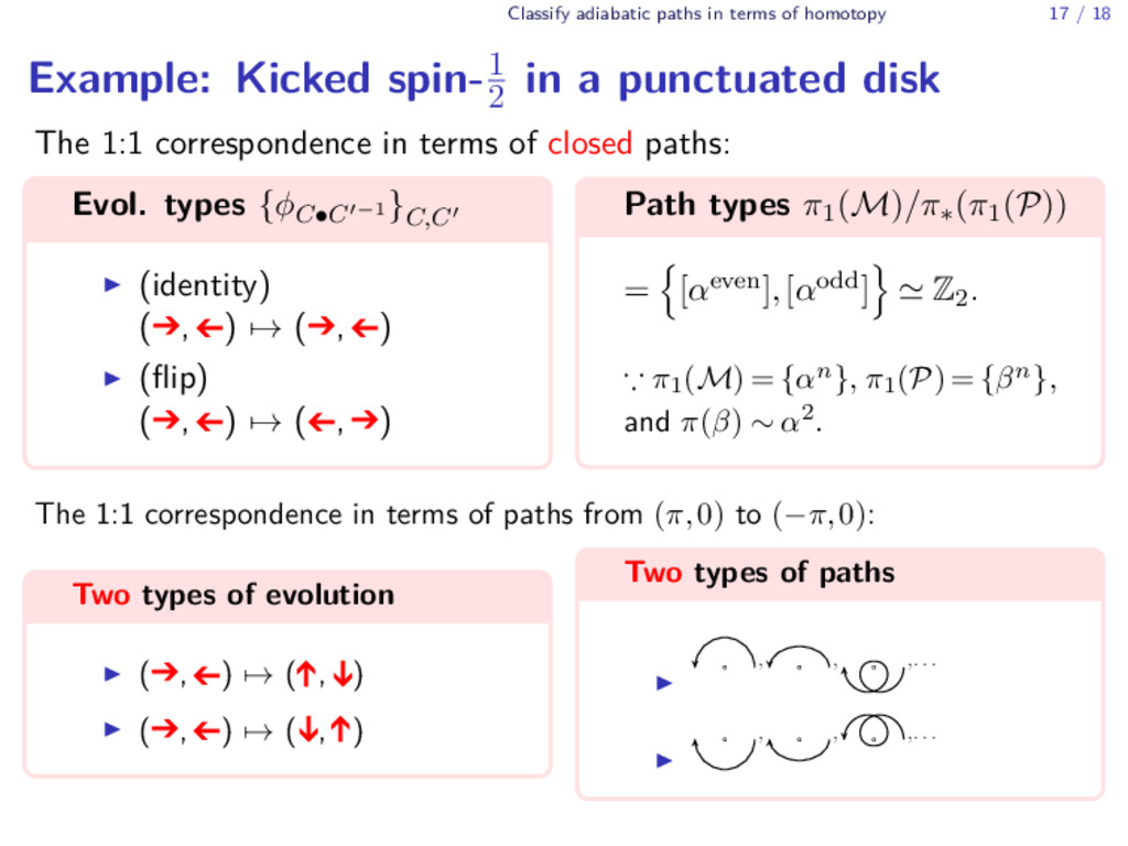
6. Introduction 6 / 18 Kicked spin: the path dependence of adiabatic evol. There are two types of adiabatic evolution for the following condition: the adiabatic path (in M) from (1,0) to (−1,0) the initial stationary state |Sx +⟩ (= ) The state of spin is depicted by the Bloch vector a (≡ ⟨σ⟩). (Type 1) the final state is |Sy +⟩ (= ) O 1 −1 |Sx + |Sy + (Type 2) the final state is |Sy −⟩ (= ) O 1 −1 |Sx + |Sy −
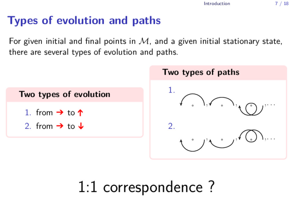
7. Introduction 7 / 18 Types of evolution and paths For given initial and final points in M, and a given initial stationary state, there are several types of evolution and paths. Two types of evolution 1. from to 2. from to Two types of paths 1. , , ,. . . 2. , , ,. . . 1:1 correspondence ?
8. Introduction 8 / 18 Aim Establish the 1:1 correspondence: Evol. types {ϕC}C Path types π1(M)/π∗(π1(P)) ▶ What is ϕC? (characterize adiabatic evolution) ▶ What is P? Note: π1(X) is the fundamental group of X.
9. Lifting adiabatic paths 9 / 18 Outline Introduction Lifting adiabatic paths Classify adiabatic paths in terms of homotopy Summary
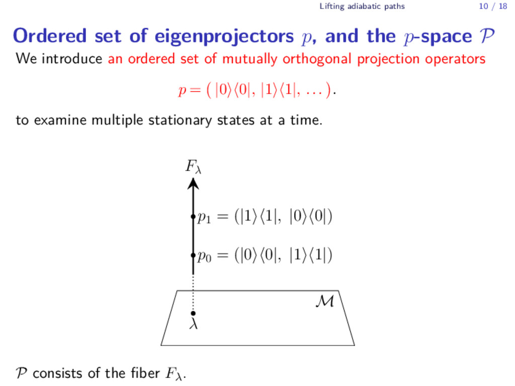
10. Lifting adiabatic paths 10 / 18 Ordered set of eigenprojectors p, and the p-space P We introduce an ordered set of mutually orthogonal projection operators p = ( |0⟩⟨0|, |1⟩⟨1|, ... ) . to examine multiple stationary states at a time. λ p0 = (|0 0|, |1 1|) p1 = (|1 1|, |0 0|) Fλ M P consists of the fiber Fλ.
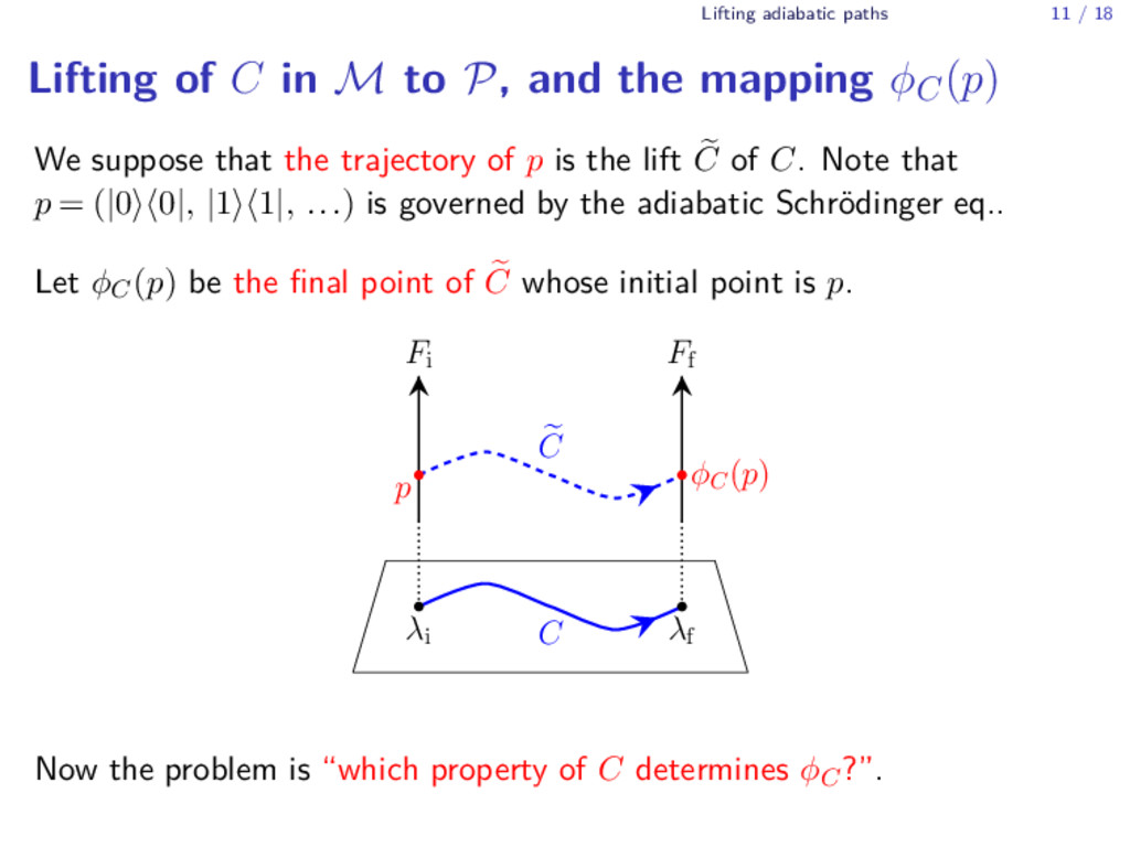
11. Lifting adiabatic paths 11 / 18 Lifting of C in M to P, and the mapping ϕC(p) We suppose that the trajectory of p is the lift C of C. Note that p = (|0⟩⟨0|, |1⟩⟨1|, ...) is governed by the adiabatic Schr¨ odinger eq.. Let ϕC(p) be the final point of C whose initial point is p. Fi Ff λi λf C p φC (p) C Now the problem is “which property of C determines ϕC?”.
12. Classify adiabatic paths in terms of homotopy 12 / 18 Outline Introduction Lifting adiabatic paths Classify adiabatic paths in terms of homotopy Summary
13. Classify adiabatic paths in terms of homotopy 13 / 18 How we study the mapping ϕC? Through the homotopic classification of C (in M) and C (in P) . The mathematical background: The projector π : P → M is called a covering projection. The covering space is a fiber bundle with a discrete structure group.
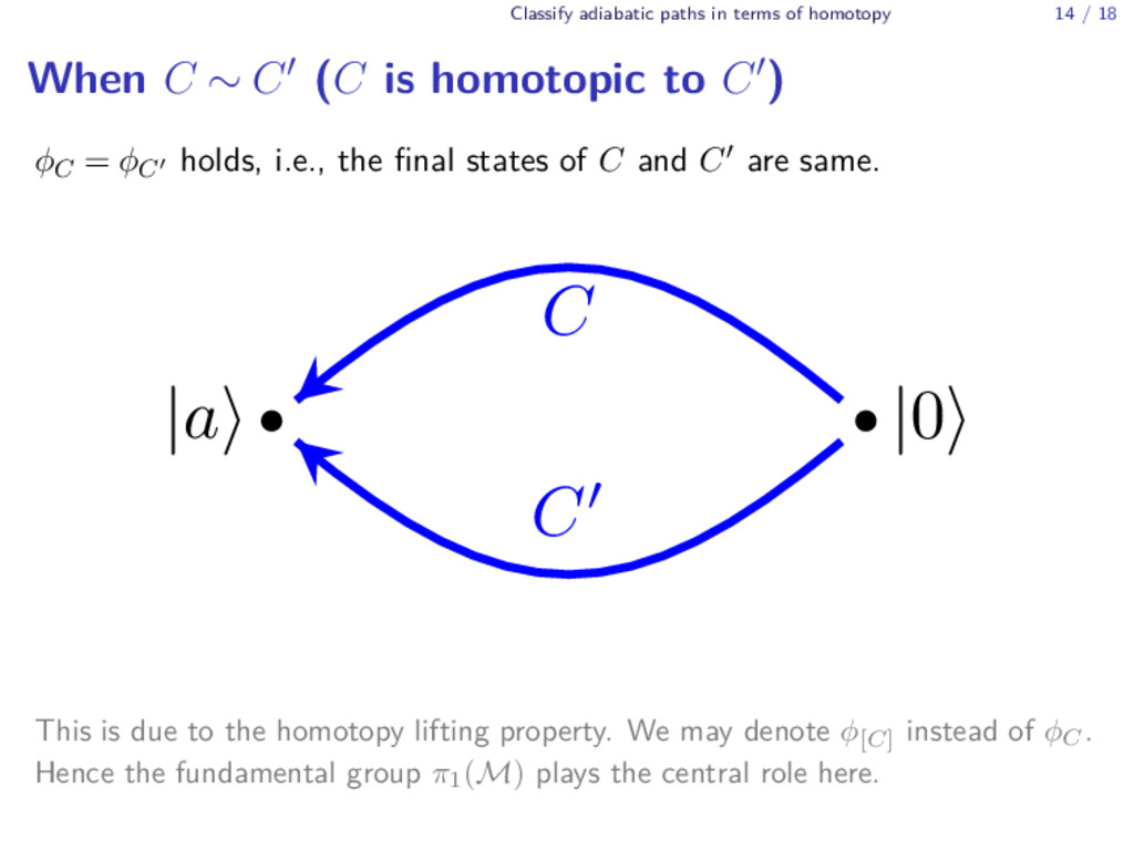
14. Classify adiabatic paths in terms of homotopy 14 / 18 When C ∼ C′ (C is homotopic to C′) ϕC = ϕC′ holds, i.e., the final states of C and C′ are same. |0 |a C C This is due to the homotopy lifting property. We may denote ϕ[C] instead of ϕC. Hence the fundamental group π1(M) plays the central role here.
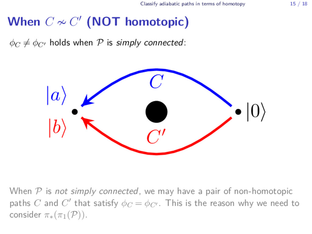
15. Classify adiabatic paths in terms of homotopy 15 / 18 When C ≁ C′ (NOT homotopic) ϕC ̸= ϕC′ holds when P is simply connected: |0 |a |b C C When P is not simply connected, we may have a pair of non-homotopic paths C and C′ that satisfy ϕC = ϕC′ . This is the reason why we need to consider π∗(π1(P)).
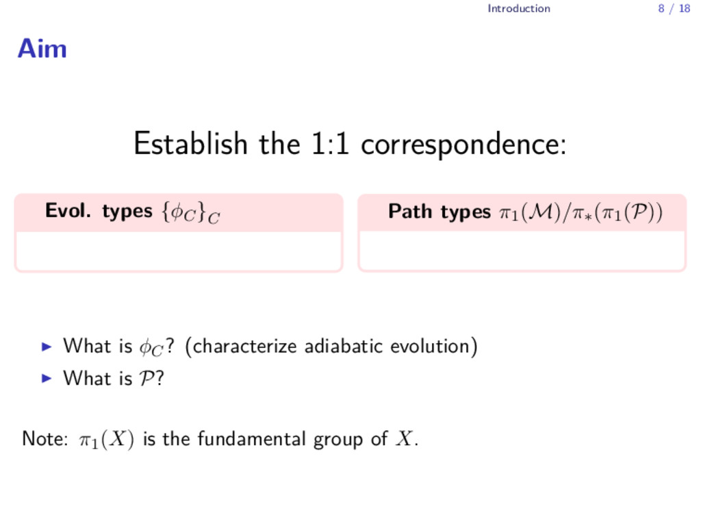
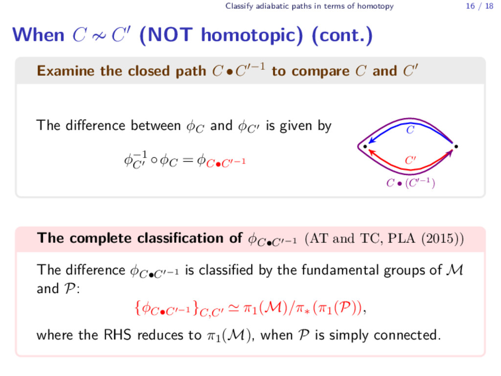
16. Classify adiabatic paths in terms of homotopy 16 / 18 When C ≁ C′ (NOT homotopic) (cont.) Examine the closed path C •C′−1 to compare C and C′ The difference between ϕC and ϕC′ is given by ϕ−1 C′ ◦ϕC = ϕC•C′−1 C C C • (C −1) The complete classification of ϕC•C′−1 (AT and TC, PLA (2015)) The difference ϕC•C′−1 is classified by the fundamental groups of M and P: {ϕC•C′−1 }C,C′ ≃ π1(M)/π∗ (π1(P)), where the RHS reduces to π1(M), when P is simply connected.
17. Classify adiabatic paths in terms of homotopy 17 / 18 Example: Kicked spin-1 2 in a punctuated disk The 1:1 correspondence in terms of closed paths: Evol. types {ϕC•C′−1 }C,C′ ▶ (identity) ( , ) → ( , ) ▶ (flip) ( , ) → ( , ) Path types π1(M)/π∗(π1(P)) = { [αeven],[αodd] } ≃ Z2. ∵ π1(M) = {αn}, π1(P) = {βn}, and π(β) ∼ α2. The 1:1 correspondence in terms of paths from (π,0) to (−π,0): Two types of evolution ▶ ( , ) → ( , ) ▶ ( , ) → ( , ) Two types of paths ▶ , , ,. . . ▶ , , ,. . .
18. Summary 18 / 18 Summary and outlook The topological aspect of the adiabatic evolution and the role of homotopic classification are clarified. The 1:1 correspondence between the evolution types and the path types is established: {ϕC•C′−1 }C,C′ ≃ π1(M)/π∗(π1(P)). Outlook ▶ Examine multiple-level systems. ▶ Extend to non-Hermitian systems (cf. H. Mehri-Dehnavi and A. Mostafazadeh (2008)) ▶ Extend to the case where the concept of the fundamental group is inapplicable (cf. TC (1998); N. Yonezawa, AT and TC (2013)). Ref. AT and TC, arXiv:1512.06983 (2015).