Hierarchy of quantum holonomies

量子ホロノミーの階層について
田中篤司(首都大理工)，全卓樹(高知工科大)
日本物理学会 2014年秋季大会の口頭講演資料 (10pAN-4)
Ref. http://researchmap.jp/jo1zufiz7-1795128/#_1795128
講演予定日 2014-09-10

Transcript

1. 1 / 15 Hierarchy of quantum holonomies ྔࢠϗϩϊϛʔͷ֊૚ʹ͍ͭͯ A. Tanaka (ాதಞ࢘) and T. Cheon (શ୎थ)A Tokyo Metoropolitan Univ. and Kochi Univ. Tech.A 2014-09-10 ೔ຊ෺ཧֶձ 2014 ೥ळقେձ (2014-09-07/10), த෦େֶ, 10pAN-4
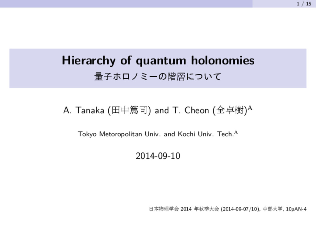
2. Introduction 2 / 15 Quantum holonomy For a given adiabatic cycle C, a closed quantum system may exhibit nontrivial response. The most famous example is the phase holonomy (a.k.a. Berry’s phase, the geometric phase) (e.g., Berry 1984). |ψ eiγ(C)|ψ eiγ(C) ˜ C C λ0 λ The phase holonomy: |ψ⟩ C − − → e−i ∫ E(t)dteiγ(C)|ψ⟩
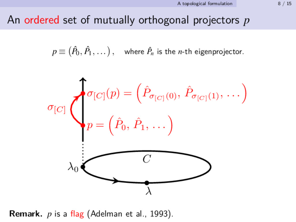
3. Introduction 3 / 15 Exotic quantum holonomy There are exotic varieties of quantum holonomy other than the geometric phase factor. A permutation of (quasi-)eigenenergies En (E0,E1,...) C − − → ( EσC(0) ,EσC(1) ,... ) , where σC(n) describes a permutation of the quantum number. A permutation of eigenprojectors ˆ Pn ≡ |n⟩⟨n| ( ˆ P0, ˆ P1,... ) C − − → ( ˆ PσC(0) , ˆ PσC(1) ,... ) Ref. TC PLA 248 (1998); AT and Miyamoto PRL 98 (2007); Yonezawa, AT and TC PRA 87 (2013) and references therein.
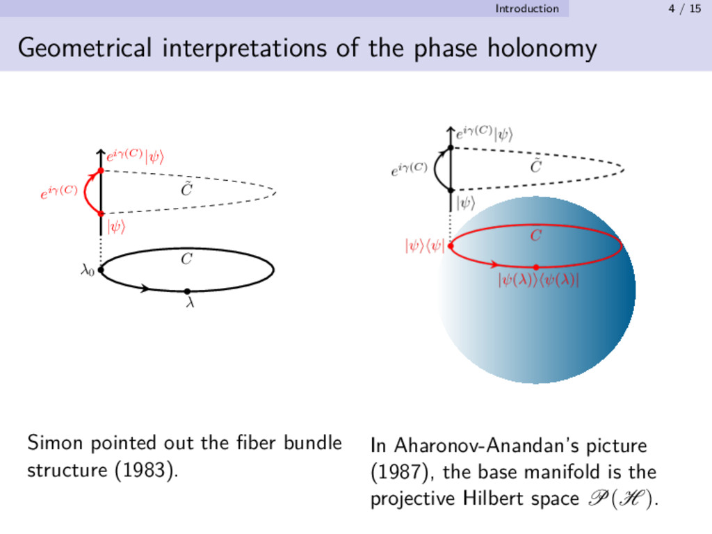
4. Introduction 4 / 15 Geometrical interpretations of the phase holonomy |ψ eiγ(C)|ψ eiγ(C) ˜ C C λ0 λ Simon pointed out the fiber bundle structure (1983). In Aharonov-Anandan’s picture (1987), the base manifold is the projective Hilbert space P(H ).
5. Introduction 5 / 15 Hierarchy of quantum holonomies |ψ f = (|0 , |1 , . . . ) ˆ P (= |ψ ψ|) p = ˆ P0 , ˆ P1 , . . . (ordered projectors) b = ˆ P0 , ˆ P1 , . . . (the order is ignored) Conventional Exotic Geometric Phase off-diagonal GP eigenspace anholonomy
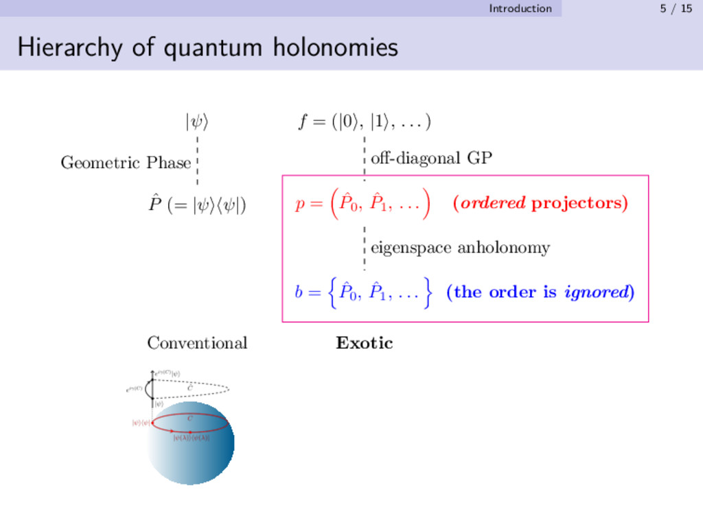
6. Introduction 6 / 15 Aim ▶ Establish a topological formulation of the eigenspace anholonomy. ▶ As for two level systems, ▶ Explain a link between the eigenspace anholonomy and disclinations of the director (headless vector) of Bloch vectors. ▶ The fundamental group of b-space (the base manifold for the exotic quantum holonomy) plays the central role. Cf. a unified treatise of the phase and eigenspace anholonomies with non-Abelian gauge connection (TC and AT EPL 85 (2009)).
7. Introduction 7 / 15 Outline Introduction A topological formulation Example in two-level systems Conclusion
8. A topological formulation 8 / 15 An ordered set of mutually orthogonal projectors p p ≡ ( ˆ P0, ˆ P1, ... ) , where ˆ Pn is the n-th eigenprojector. p = ˆ P0 , ˆ P1 , . . . σ[C] (p) = ˆ Pσ[C] (0) , ˆ Pσ[C] (1) , . . . σ[C] C λ0 λ Remark. p is a flag (Adelman et al., 1993).
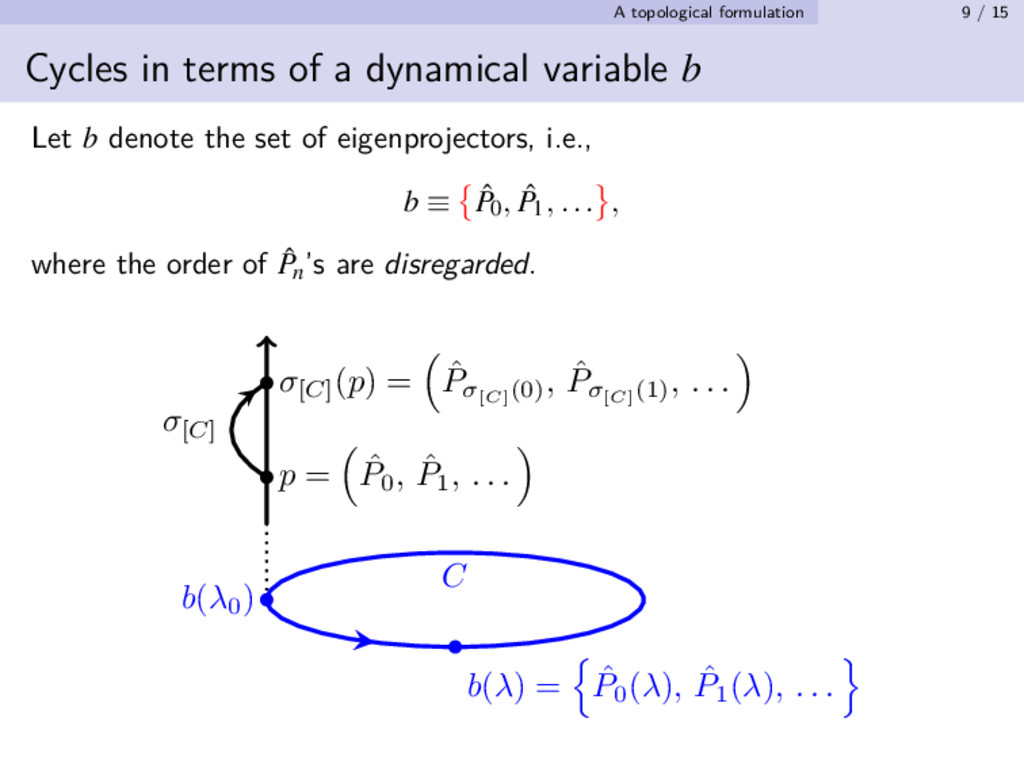
9. A topological formulation 9 / 15 Cycles in terms of a dynamical variable b Let b denote the set of eigenprojectors, i.e., b ≡ { ˆ P0, ˆ P1, ... } , where the order of ˆ Pn ’s are disregarded. p = ˆ P0 , ˆ P1 , . . . σ[C] (p) = ˆ Pσ[C] (0) , ˆ Pσ[C] (1) , . . . σ[C] C b(λ0 ) b(λ) = ˆ P0 (λ), ˆ P1 (λ), . . .
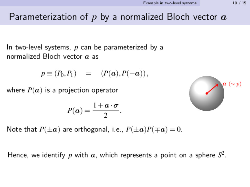
10. Example in two-level systems 10 / 15 Parameterization of p by a normalized Bloch vector a In two-level systems, p can be parameterized by a normalized Bloch vector a as p ≡ (P0,P1) = (P(a),P(−a)), where P(a) is a projection operator P(a) = 1+a·σ 2 . Note that P(±a) are orthogonal, i.e., P(±a)P(∓a) = 0. a (∼ p) Hence, we identify p with a, which represents a point on a sphere S2.
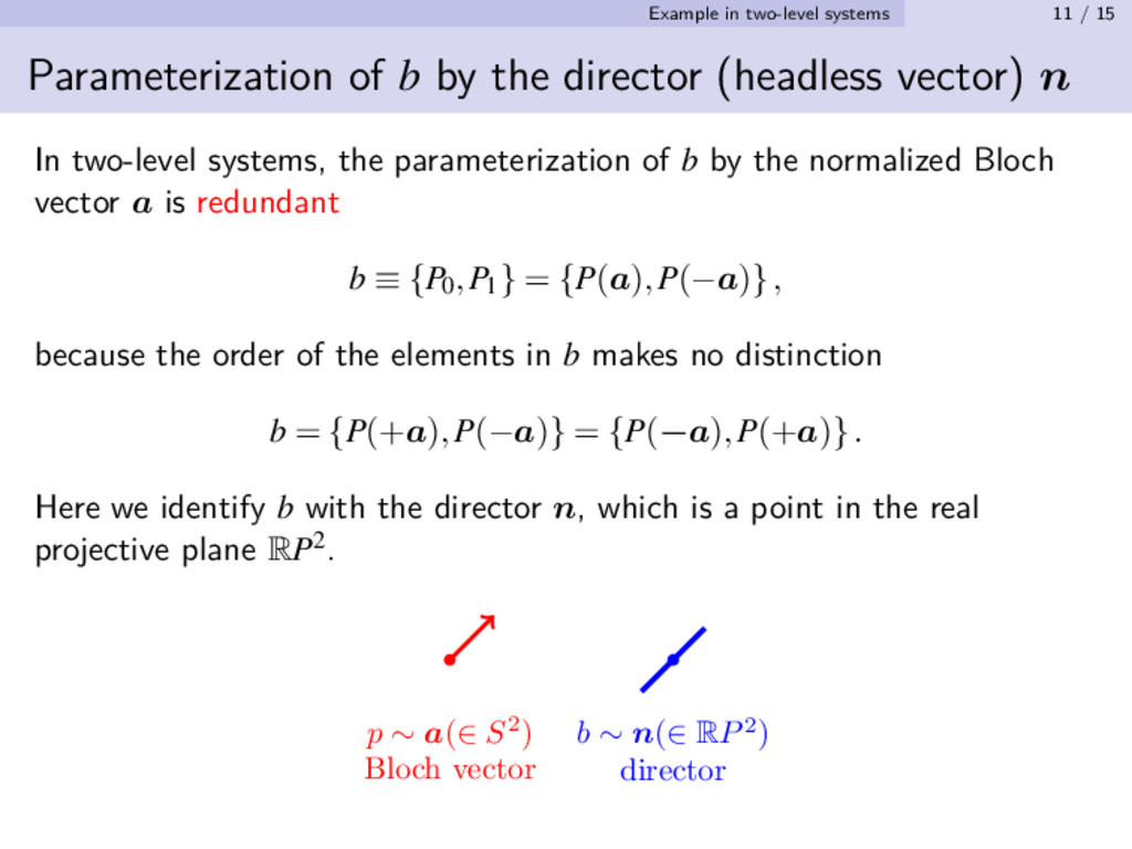
11. Example in two-level systems 11 / 15 Parameterization of b by the director (headless vector) n In two-level systems, the parameterization of b by the normalized Bloch vector a is redundant b ≡ {P0,P1} = {P(a),P(−a)}, because the order of the elements in b makes no distinction b = {P(+a),P(−a)} = {P(−a),P(+a)}. Here we identify b with the director n, which is a point in the real projective plane RP2. p ∼ a(∈ S2) Bloch vector b ∼ n(∈ RP2) director
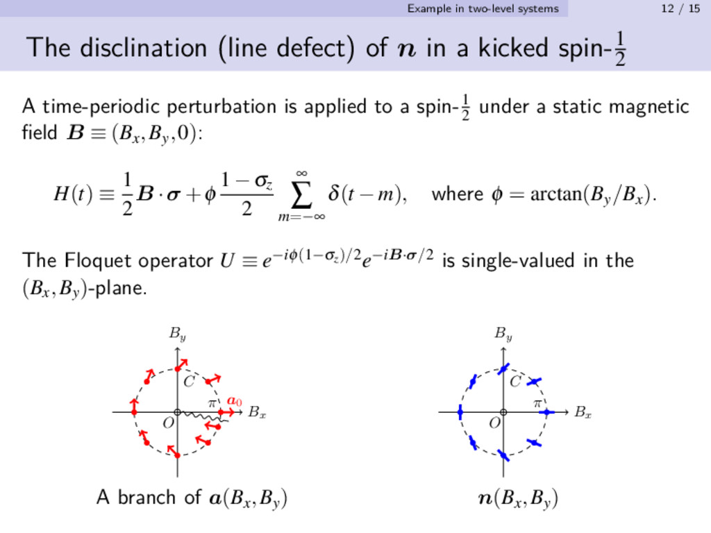
12. Example in two-level systems 12 / 15 The disclination (line defect) of n in a kicked spin-1 2 A time-periodic perturbation is applied to a spin-1 2 under a static magnetic field B ≡ (Bx,By,0): H(t) ≡ 1 2 B ·σ +ϕ 1−σz 2 ∞ ∑ m=−∞ δ(t −m), where ϕ = arctan(By/Bx). The Floquet operator U ≡ e−iϕ(1−σz)/2e−iB·σ/2 is single-valued in the (Bx,By)-plane. Bx By O C π a0 A branch of a(Bx,By) Bx By O π C n(Bx,By)
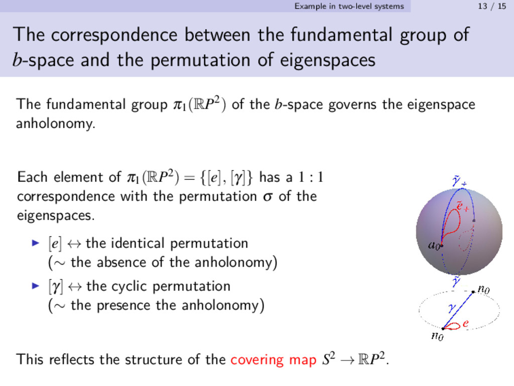
13. Example in two-level systems 13 / 15 The correspondence between the fundamental group of b-space and the permutation of eigenspaces The fundamental group π1(RP2) of the b-space governs the eigenspace anholonomy. Each element of π1(RP2) = {[e], [γ]} has a 1 : 1 correspondence with the permutation σ of the eigenspaces. ▶ [e] ↔ the identical permutation (∼ the absence of the anholonomy) ▶ [γ] ↔ the cyclic permutation (∼ the presence the anholonomy) This reflects the structure of the covering map S2 → RP2.
14. Conclusion 14 / 15 Corollary and outlook Corollary ▶ It is straightforward to obtain a nonadiabatic extension, when the cycle is parameterized by b (cf. Aharonov and Anandan 1987). Outlook ▶ Analysis of N-dimensional systems. ▶ Analysis of nonhermitian systems. Cf. exotic quantum holonomy in terms of Kato’s exceptional points (Kim, TC and AT PLA 2010, Yonezawa, AT, and TC PRA 2013, AT, Kim and TC PRE 2014).
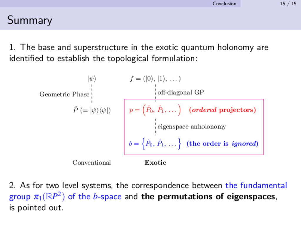
15. Conclusion 15 / 15 Summary 1. The base and superstructure in the exotic quantum holonomy are identified to establish the topological formulation: |ψ f = (|0 , |1 , . . . ) ˆ P (= |ψ ψ|) p = ˆ P0 , ˆ P1 , . . . (ordered projectors) b = ˆ P0 , ˆ P1 , . . . (the order is ignored) Conventional Exotic Geometric Phase off-diagonal GP eigenspace anholonomy 2. As for two level systems, the correspondence between the fundamental group π1(RP2) of the b-space and the permutations of eigenspaces, is pointed out.