Interrupt me. • Raising Hand, Speak Up, etc… From Me: • I will randomly pick someone using the numbers you were given. We will not move on until we can sum up the question. (no man/woman left behind) • I need someone to record the questions and answers given during the class so that I can verify the answers and redistribute them as review material.
a Modern Approach (AIMA) 2nd Edition (CH6) • AIMA 3rd Edition (CH5) • Game Theory for Applied Economics • Robert Gibson (Princeton University Press) • PDF (pre-print) Available on request.
View actors of problems as agents (ch2) • View problems as games (game theory) • Recursion (Basic Computer Science) • New Knowledge: • Use searching to “win” games.
The “thing” trying to solve the problem. • It perceives and acts in its environment. • An “agent function” is the agents response to a “percept sequence” • Performance measures determine how “well” the agent is doing (happiness). • Reflex vs. Model Based. • Room for improvement through learning (See this in a later course)
Representing a “real” world scenario and all of the possible decisions. • Multi-Agent! • Mapping decisions (agent functions) to outcomes (performance measures) • Trying to pick a grouping of decisions that lead to the best possible outcome (not always winning)
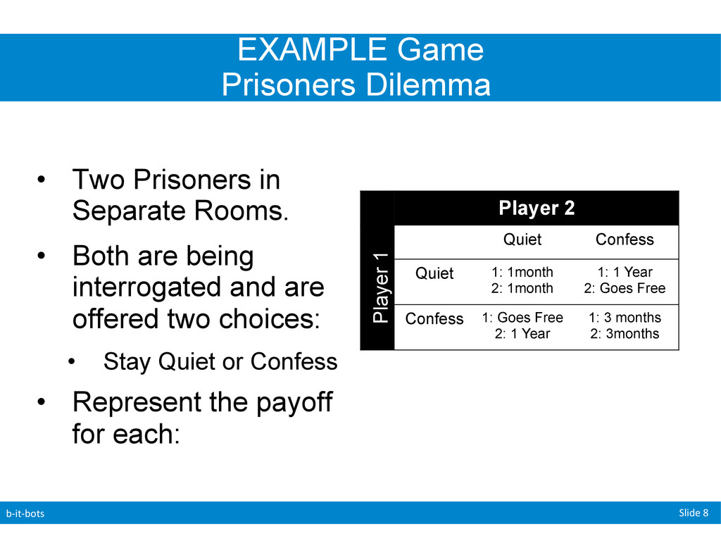
Two Prisoners in Separate Rooms. • Both are being interrogated and are offered two choices: • Stay Quiet or Confess • Represent the payoff for each: Player 2 Player 1 Quiet Confess Quiet 1: 1month 2: 1month 1: 1 Year 2: Goes Free Confess 1: Goes Free 2: 1 Year 1: 3 months 2: 3months
We can no longer make decisions the same way we did before. • We need to consider what the other players (agent(s)) might do. • This will affect our searching strategies!
searching through the state-space for a specific type of games namely: • Game Theory: • Two Player, Deterministic, co-operative/competitive, Turn taking, Zero-sum Games of Perfect Information. • Artificial Intelligence: • Two-Agent, Deterministic, (competitive), Turn Taking, Zero-sum, Fully Observable
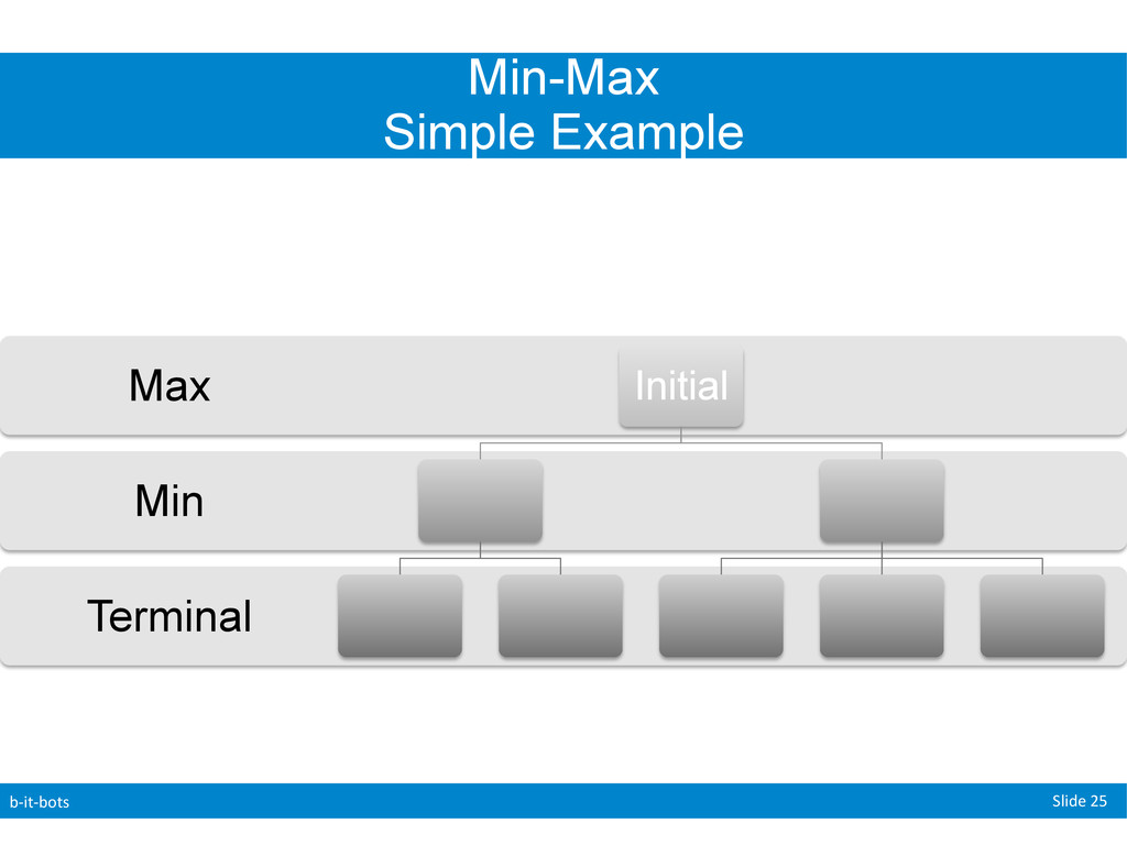
Game: • A Search problem that contains the following elements: • Initial State • Player(s) • Action(s) • Result(s) • Terminal Test • Utility Function (payoff function, objective function)
going with this: • Min-Max Search Algorithm • Alpha-Beta Search Algorithm • Heavy focus on parsing with this one! • Chance & Imperfection • If we have time • !!You still need to cover this for the course!!
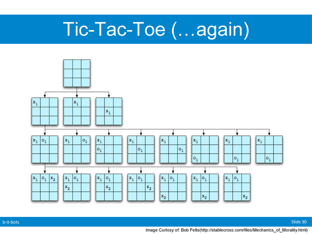
was a “small” game. • Two players, Two Options • 4 possible outcomes • A possible outcome is called a “Terminal State” • AIMA looks at another “small” game: • Tic-Tac-Toe • 362880 Terminal Nodes • Chess has 1040 Terminal Nodes!
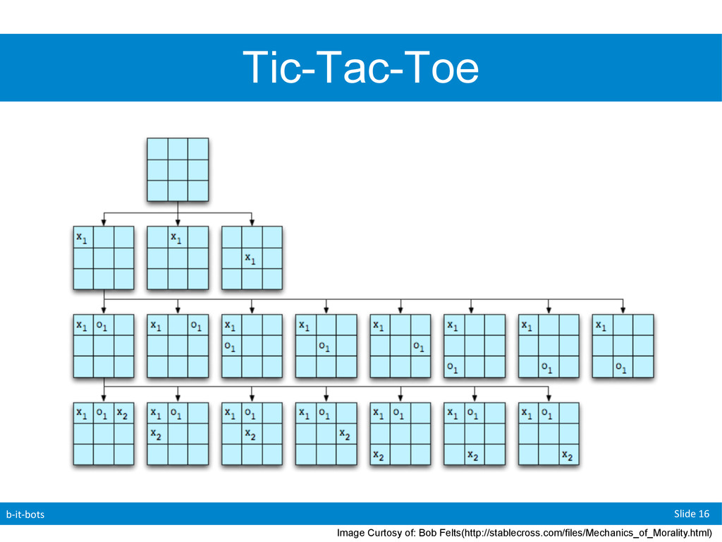
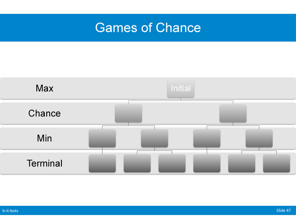
Before when we used a search tree we would examined the “whole” state space • In games we do not have this luxury. • For now we will describe search trees as a tree that is “super-imposed” on our state space that allows us to see enough nodes in order to allow a player to determine their next move
two-person zero-sum game with finitely many strategies there exists a value V and a mixed strategy for each player such that: ① Given Player 2’s strategy, the best payoff possible for player 1 is V and ② Given Player 1’s strategy, the best payoff possible for player 2 is -V
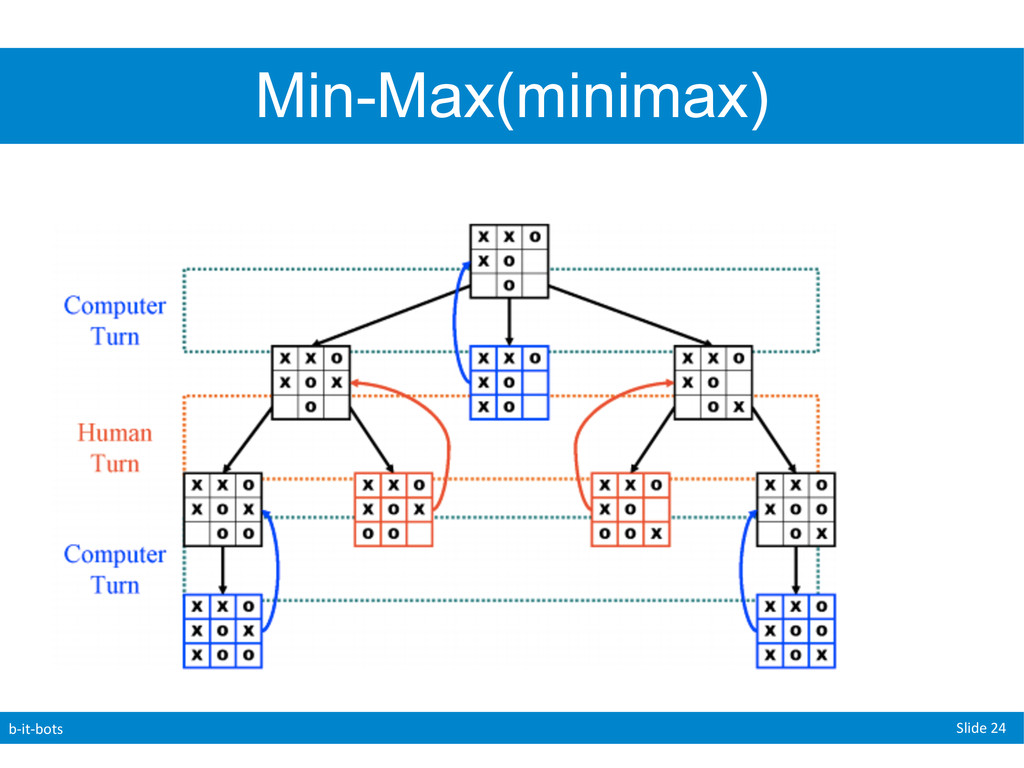
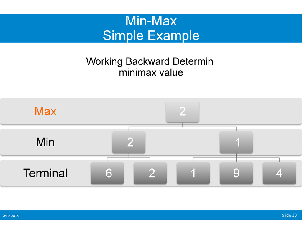
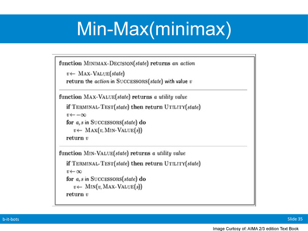
players ( “min” & “max”(us)) • Now we need to generate the state space • Recursively generate all possible moves for each turn until we reach a game ending. • Given three possible states (-1,1,0) • -1: lose, 1:win 0: draw • Max (we) will try to maximize the game score • Eg: game score -> 1 • Min will try to minimize the game score • Eg: game score -> -1
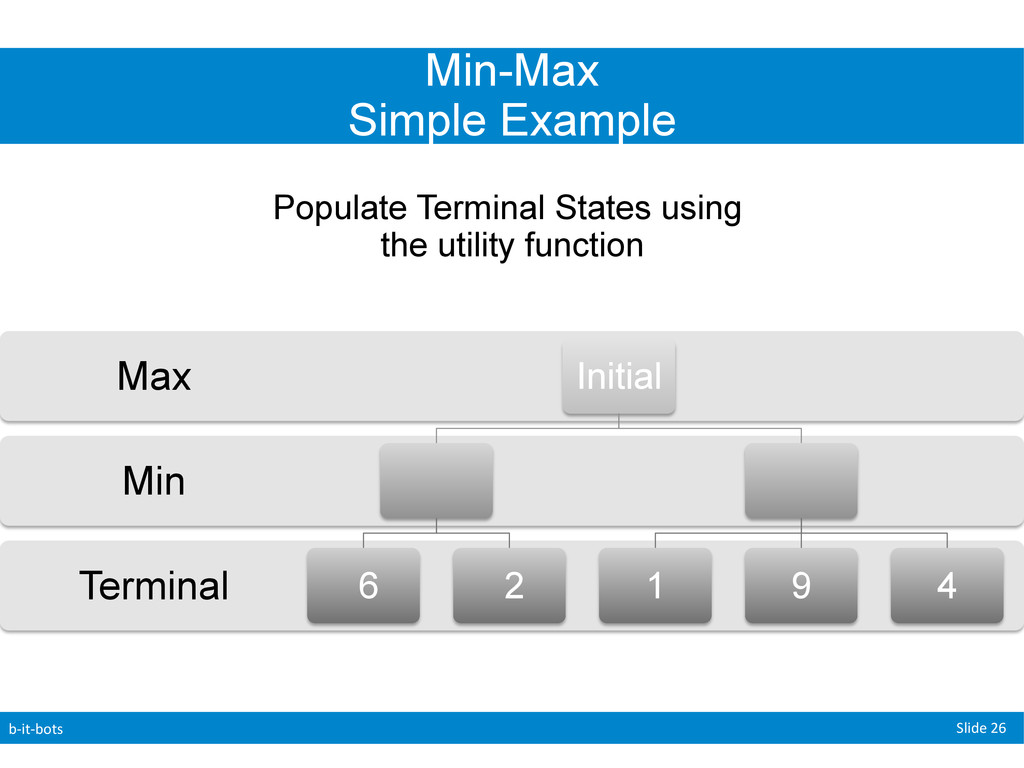
a “value” to the final possible boards (1,0,-1) • Note: This value does not have to be 1,0,-1 I simply picked these values to demonstrate my point. • How do we assign values along the way? (eg: from our initial to our goal state) • Keep in mind that for now both players are perfect.
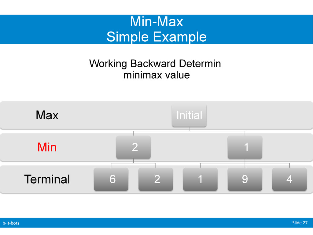
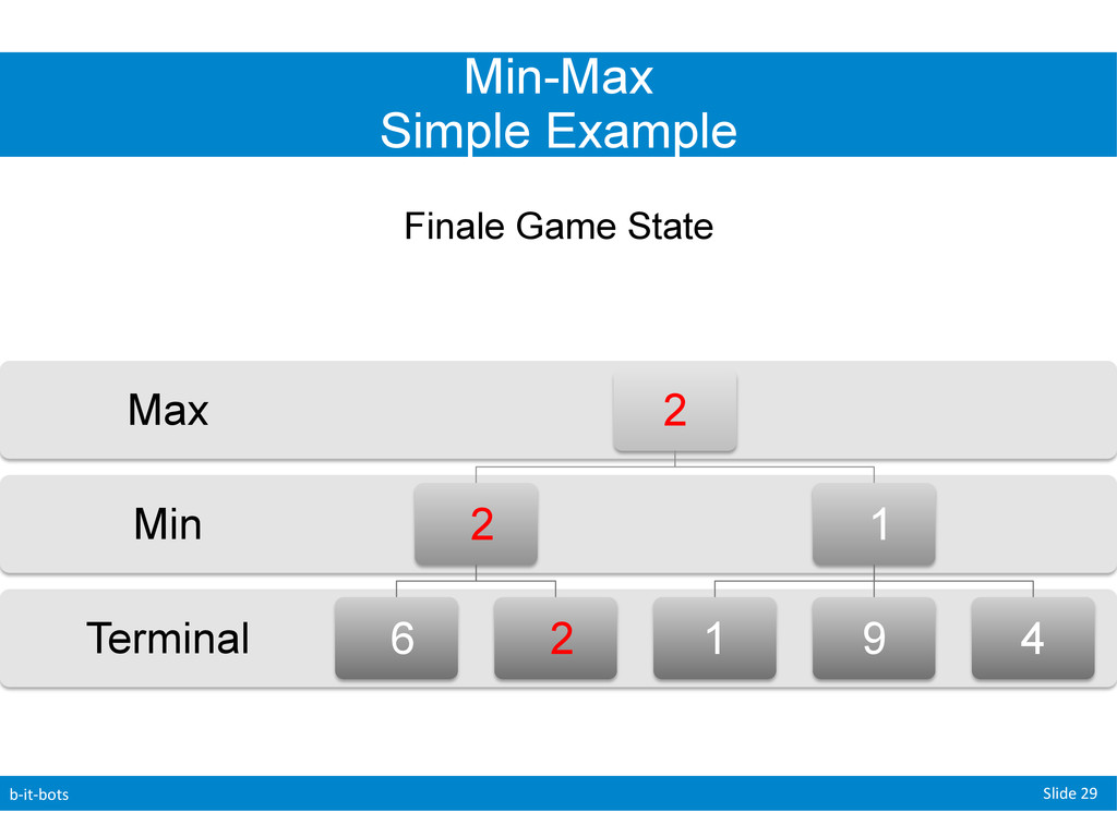
is perfect they will always make the best decision for themselves at that point. • To deal with this we will simply give each “game” (board) the best possible value that can result from any of the moves that can be made from the current location. • We do this recursively by starting at the end position and propagating values “upwards” • Note that the branching factor can commonly change from one move to another as one players moves affects the possible moves of the other
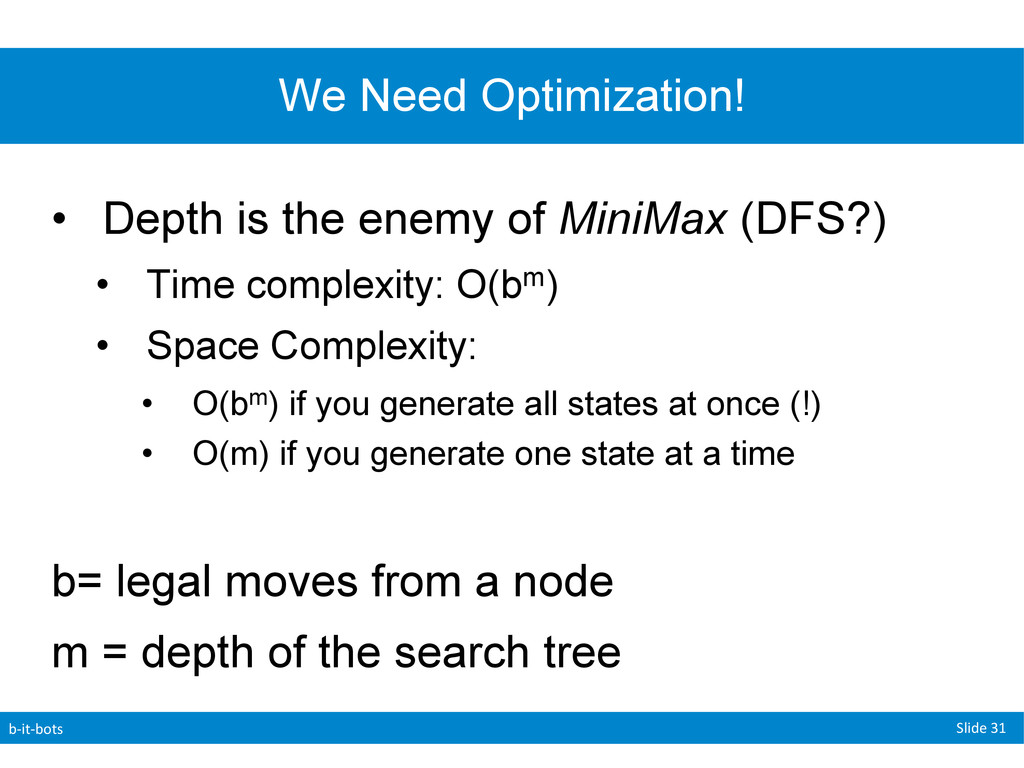
is the enemy of MiniMax (DFS?) • Time complexity: O(bm) • Space Complexity: • O(bm) if you generate all states at once (!) • O(m) if you generate one state at a time b= legal moves from a node m = depth of the search tree
simple optimization. • Given the same game, it must reach the same decision as minimax. • It will not however generate states or branches that can have no effect on the end result.
called α-β Pruning because of the following parameters: • α = the value of the best (i.e., highest-value) choice we have found so far at any choice point along the path for MAX. • β = the value of the best (i.e., lowest-value) choice we have found so far at any choice point along the path for MIN.
will search through the tree updating the values for α and β. • If the value of a current node is worse than α or β for Max or Min (respectively) we “prune” the search tree • In this case pruning means we terminate that particular recursive call.
Tables • A hash map off all the positions that we have been in before. As noted earlier revisiting nodes can cause an exponential explosion in both time and space complexity. We can use transposition tables to avoid this increase.
Minimax • Helps us deal with opponents (but is time and space cost inefficient). • α-β Pruning • Helps us deal with the space and time costs of MiniMax But α-β still requires us to search to the terminal states!
do not have the time or power to search a full tree before a decision can be made this leads us into the realm of imperfect decision making • Note: This is not guessing (we are not there yet…)
evaluate terminal states in the same way that the utility function does. 2. Computation must be fast (the whole point now is speed!) 3. For nonterminal states our EVAL should be pretty closely tied to our chances of winning • This is typically done through weighted linear functions (read AIMA for more!)
these techniques you employ the “smarter” your algorithms become. • But be warned! • They are more prone to errors! Each method approximates some aspect instead of fully investigating it
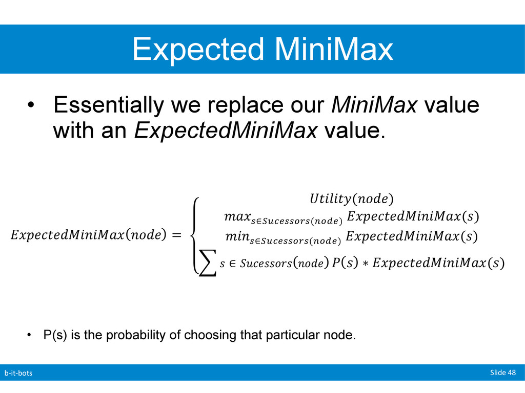
replace our MiniMax value with an ExpectedMiniMax value. • P(s) is the probability of choosing that particular node. !"#$%&$'()*)(+" !"#$ =! !"#$#"%(!"#$) !"# !∈!"#$%%&'%(!"#$) !!"#$%&$'()*)(+"(!) !"# !∈!"#$%%&'%(!"#$) !!"#$%&$'()*)(+"(!) ! ∈ !"#$%%&'% !"#$ ! ! ∗ !"#$%&$'()*)(+"(!) !!
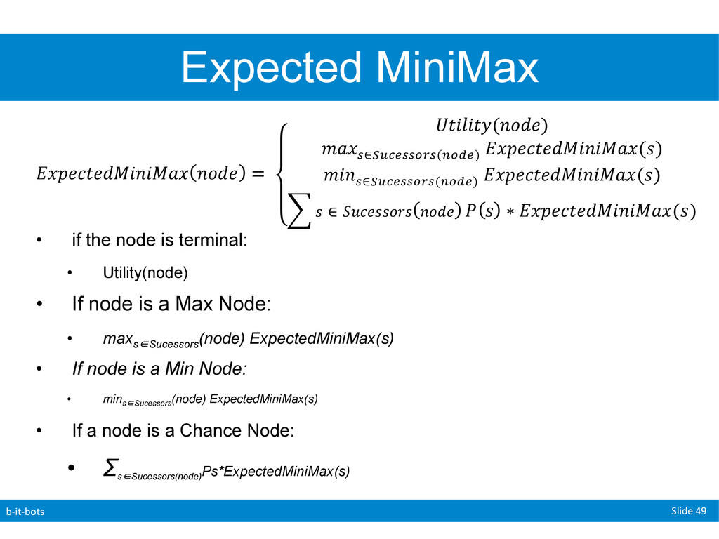
node is terminal: • Utility(node) • If node is a Max Node: • maxs∈Sucessors (node) ExpectedMiniMax(s) • If node is a Min Node: • mins∈Sucessors (node) ExpectedMiniMax(s) • If a node is a Chance Node: • Σ s∈Sucessors(node) Ps*ExpectedMiniMax(s) !"#$%&$'()*)(+" !"#$ =! !"#$#"%(!"#$) !"# !∈!"#$%%&'%(!"#$) !!"#$%&$'()*)(+"(!) !"# !∈!"#$%%&'%(!"#$) !!"#$%&$'()*)(+"(!) ! ∈ !"#$%%&'% !"#$ ! ! ∗ !"#$%&$'()*)(+"(!) !!
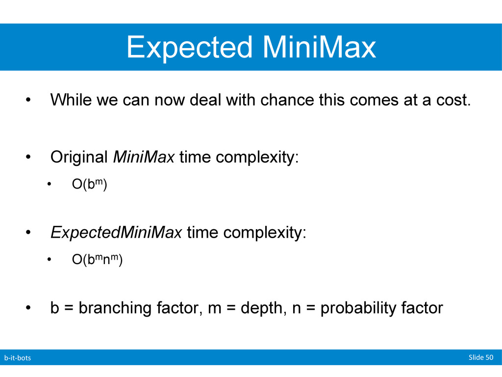
can now deal with chance this comes at a cost. • Original MiniMax time complexity: • O(bm) • ExpectedMiniMax time complexity: • O(bmnm) • b = branching factor, m = depth, n = probability factor
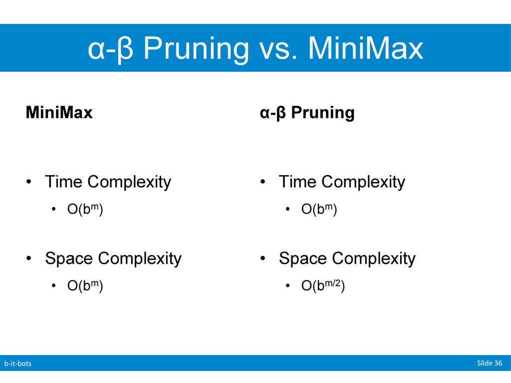
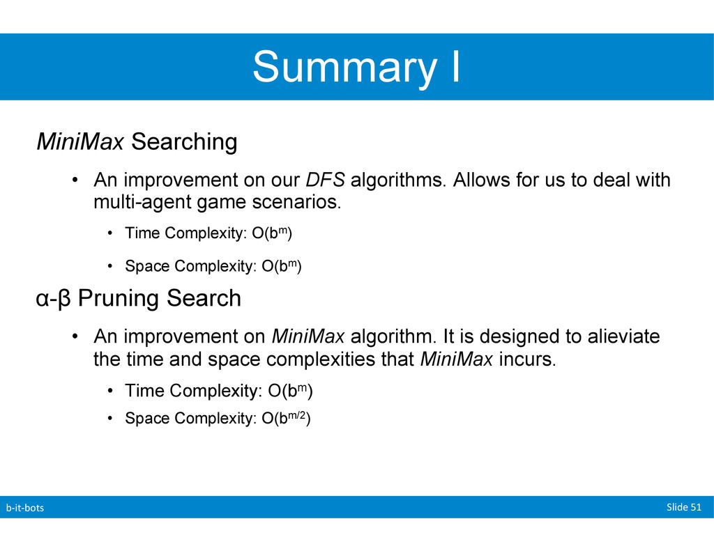
An improvement on our DFS algorithms. Allows for us to deal with multi-agent game scenarios. • Time Complexity: O(bm) • Space Complexity: O(bm) α-β Pruning Search • An improvement on MiniMax algorithm. It is designed to alieviate the time and space complexities that MiniMax incurs. • Time Complexity: O(bm) • Space Complexity: O(bm/2)
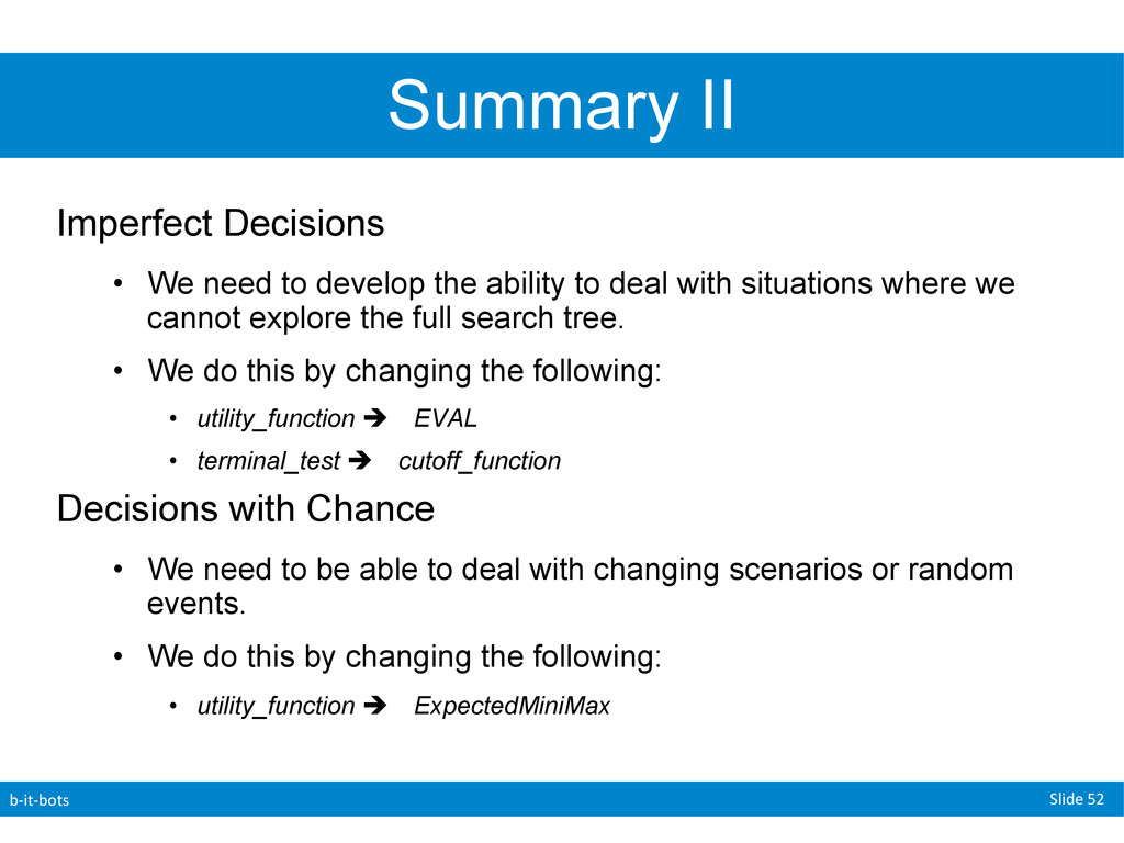
We need to develop the ability to deal with situations where we cannot explore the full search tree. • We do this by changing the following: • utility_function è EVAL • terminal_test è cutoff_function Decisions with Chance • We need to be able to deal with changing scenarios or random events. • We do this by changing the following: • utility_function è ExpectedMiniMax
Create an ant that is able to survive, reproduce, and conquer the other ants! • We will work on it during the lab session as well as an assignment. • You can play against each other very easily! • Work in groups of 2! • http://www.aichallenge.org
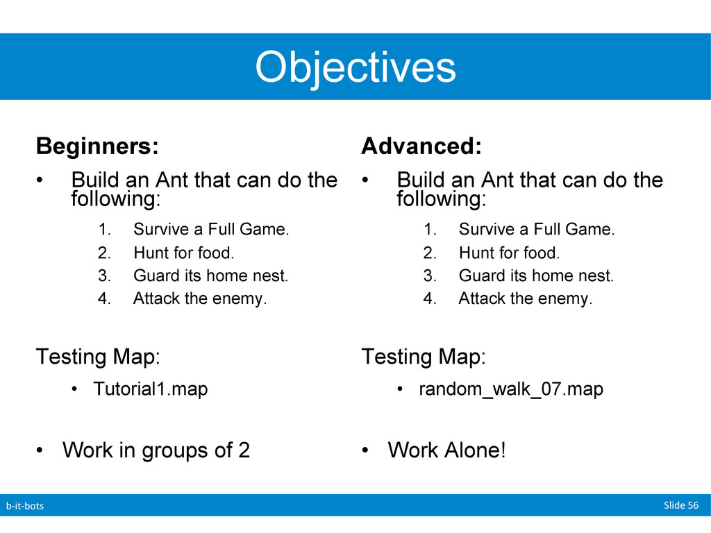
Ant that can do the following: 1. Survive a Full Game. 2. Hunt for food. 3. Guard its home nest. 4. Attack the enemy. Testing Map: • Tutorial1.map • Work in groups of 2 Advanced: • Build an Ant that can do the following: 1. Survive a Full Game. 2. Hunt for food. 3. Guard its home nest. 4. Attack the enemy. Testing Map: • random_walk_07.map • Work Alone!
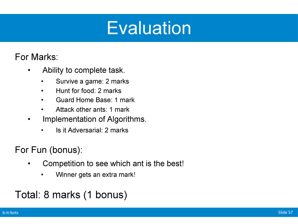
to complete task. • Survive a game: 2 marks • Hunt for food: 2 marks • Guard Home Base: 1 mark • Attack other ants: 1 mark • Implementation of Algorithms. • Is it Adversarial: 2 marks For Fun (bonus): • Competition to see which ant is the best! • Winner gets an extra mark! Total: 8 marks (1 bonus)