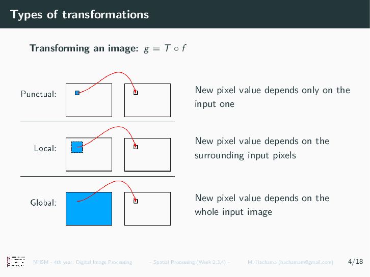
f New pixel value depends only on the input one New pixel value depends on the surrounding input pixels New pixel value depends on the whole input image NHSM - 4th year: Digital Image Processing - Spatial Processing (Week 2,3,4) - M. Hachama ([email protected]) 4/18
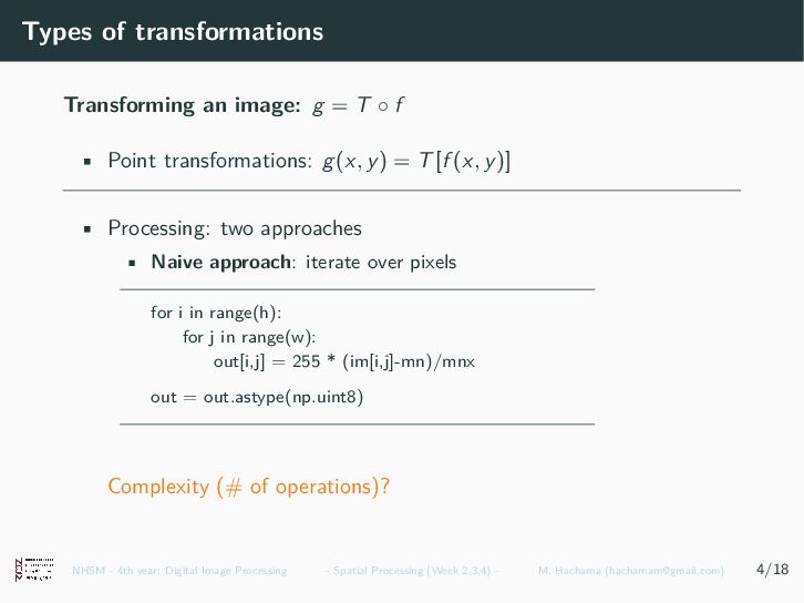
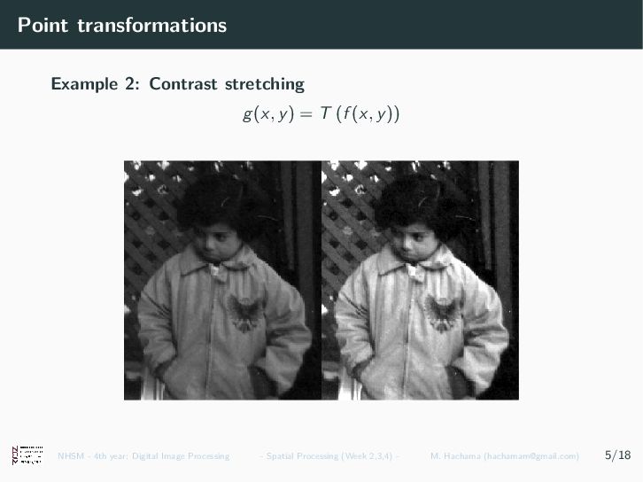
f • Point transformations: g(x, y) = T[f (x, y)] • Processing: two approaches • Naive approach: iterate over pixels for i in range(h): for j in range(w): out[i,j] = 255 * (im[i,j]-mn)/mnx out = out.astype(np.uint8) Complexity (# of operations)? NHSM - 4th year: Digital Image Processing - Spatial Processing (Week 2,3,4) - M. Hachama ([email protected]) 4/18
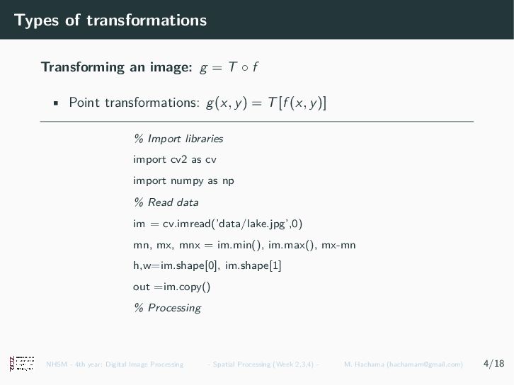
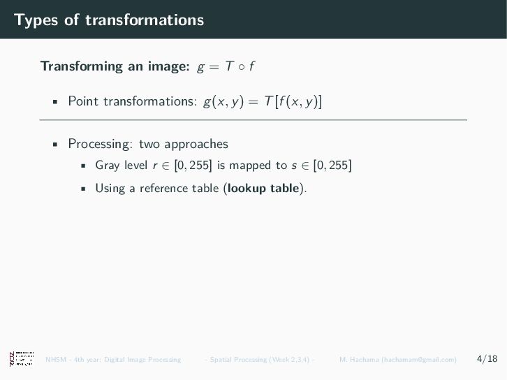
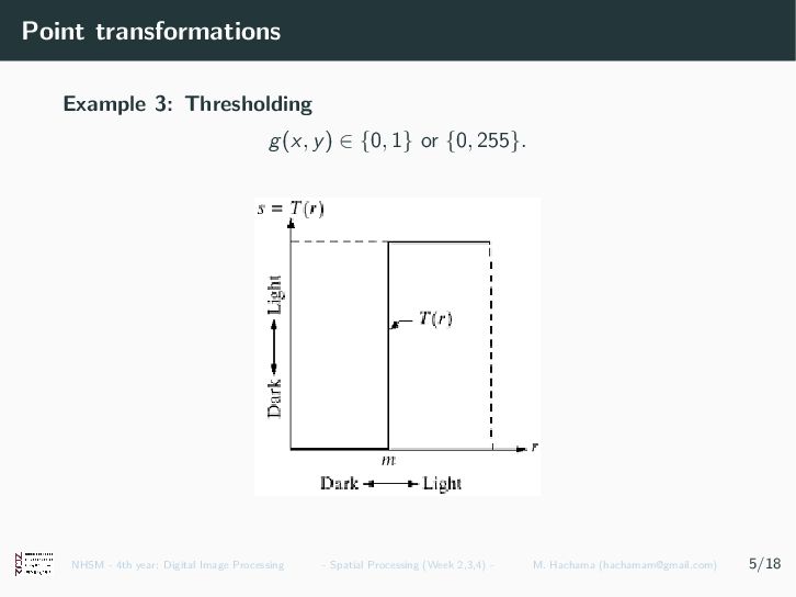
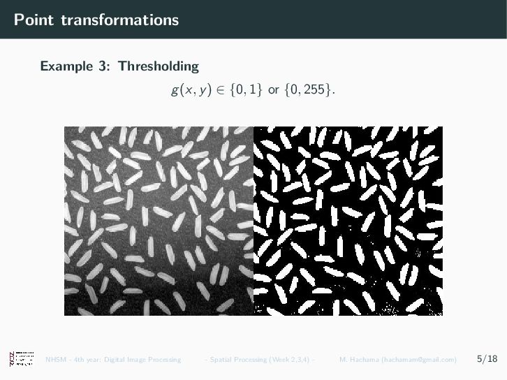
f • Point transformations: g(x, y) = T[f (x, y)] • Processing: two approaches • Gray level r ∈ [0, 255] is mapped to s ∈ [0, 255] • Using a reference table (lookup table). NHSM - 4th year: Digital Image Processing - Spatial Processing (Week 2,3,4) - M. Hachama ([email protected]) 4/18
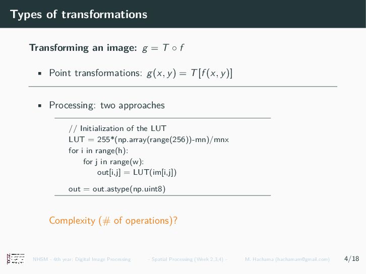
f • Point transformations: g(x, y) = T[f (x, y)] • Processing: two approaches // Initialization of the LUT LUT = 255*(np.array(range(256))-mn)/mnx for i in range(h): for j in range(w): out[i,j] = LUT(im[i,j]) out = out.astype(np.uint8) Complexity (# of operations)? NHSM - 4th year: Digital Image Processing - Spatial Processing (Week 2,3,4) - M. Hachama ([email protected]) 4/18
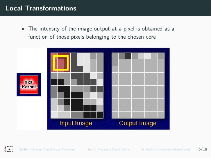
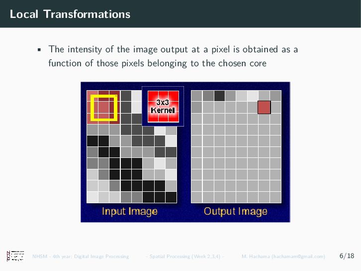
a pixel is obtained as a function of those pixels belonging to the chosen core NHSM - 4th year: Digital Image Processing - Spatial Processing (Week 2,3,4) - M. Hachama ([email protected]) 6/18
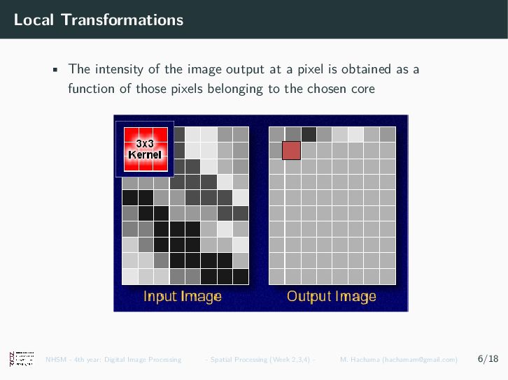
a pixel is obtained as a function of those pixels belonging to the chosen core NHSM - 4th year: Digital Image Processing - Spatial Processing (Week 2,3,4) - M. Hachama ([email protected]) 6/18
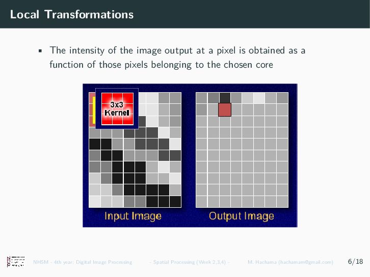
a pixel is obtained as a function of those pixels belonging to the chosen core NHSM - 4th year: Digital Image Processing - Spatial Processing (Week 2,3,4) - M. Hachama ([email protected]) 6/18
a pixel is obtained as a function of those pixels belonging to the chosen core NHSM - 4th year: Digital Image Processing - Spatial Processing (Week 2,3,4) - M. Hachama ([email protected]) 6/18
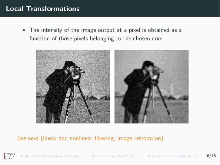
a pixel is obtained as a function of those pixels belonging to the chosen core See next (linear and nonlinear filtering, image restoration) NHSM - 4th year: Digital Image Processing - Spatial Processing (Week 2,3,4) - M. Hachama ([email protected]) 6/18
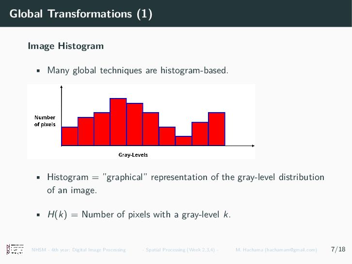
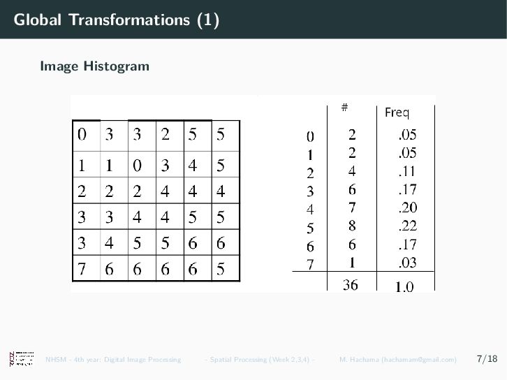
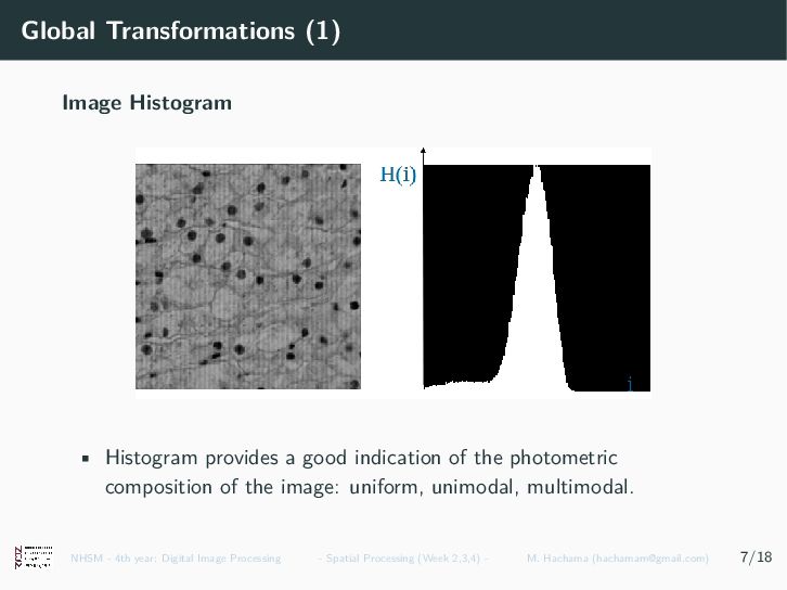
histogram-based. • Histogram = ”graphical” representation of the gray-level distribution of an image. • H(k) = Number of pixels with a gray-level k. NHSM - 4th year: Digital Image Processing - Spatial Processing (Week 2,3,4) - M. Hachama ([email protected]) 7/18
indication of the photometric composition of the image: uniform, unimodal, multimodal. NHSM - 4th year: Digital Image Processing - Spatial Processing (Week 2,3,4) - M. Hachama ([email protected]) 7/18
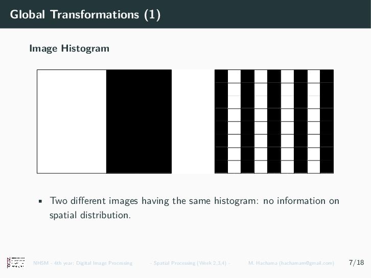
the same histogram: no information on spatial distribution. NHSM - 4th year: Digital Image Processing - Spatial Processing (Week 2,3,4) - M. Hachama ([email protected]) 7/18
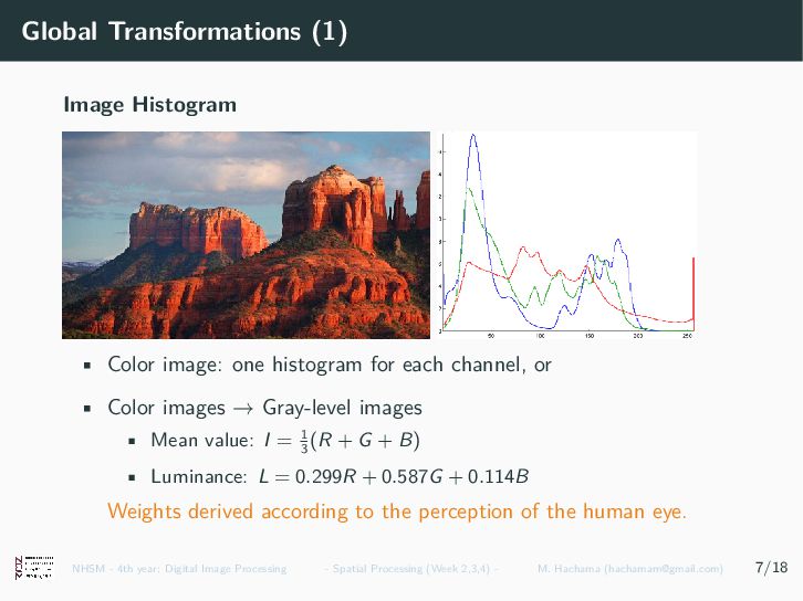
for each channel, or • Color images → Gray-level images • Mean value: I = 1 3 (R + G + B) • Luminance: L = 0.299R + 0.587G + 0.114B Weights derived according to the perception of the human eye. NHSM - 4th year: Digital Image Processing - Spatial Processing (Week 2,3,4) - M. Hachama ([email protected]) 7/18
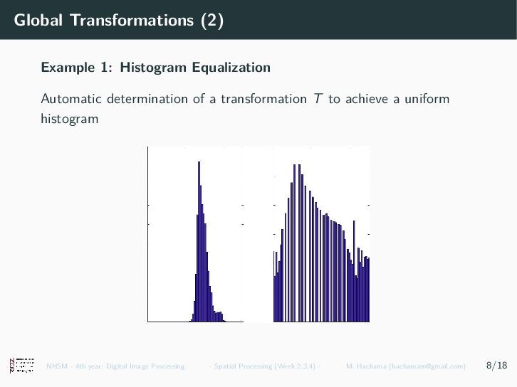
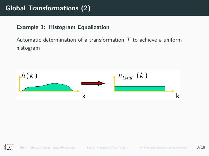
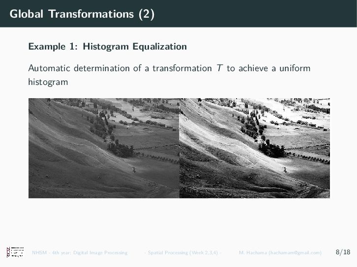
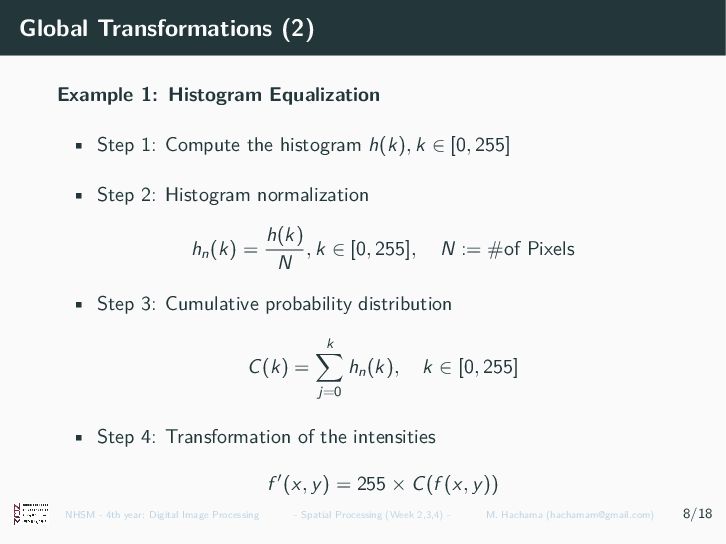
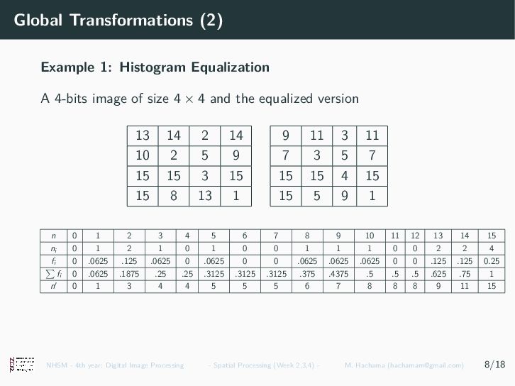
a transformation T to achieve a uniform histogram NHSM - 4th year: Digital Image Processing - Spatial Processing (Week 2,3,4) - M. Hachama ([email protected]) 8/18
a transformation T to achieve a uniform histogram NHSM - 4th year: Digital Image Processing - Spatial Processing (Week 2,3,4) - M. Hachama ([email protected]) 8/18
a transformation T to achieve a uniform histogram NHSM - 4th year: Digital Image Processing - Spatial Processing (Week 2,3,4) - M. Hachama ([email protected]) 8/18
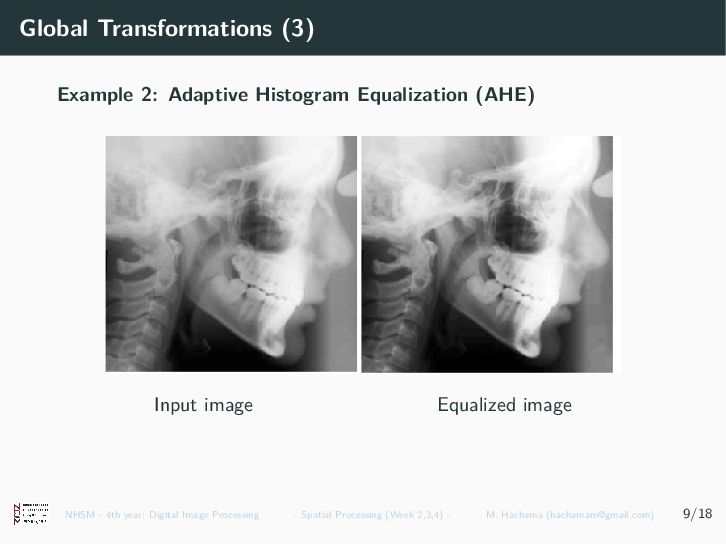
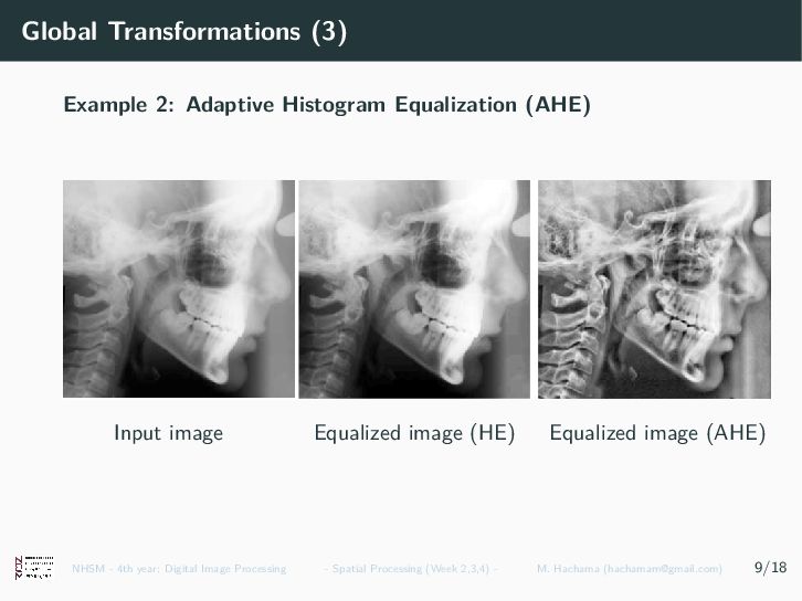
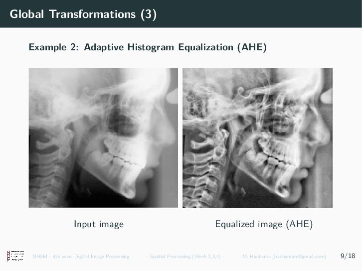
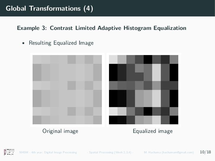
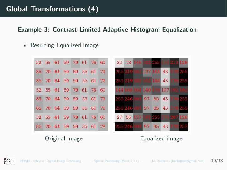
image Equalized image Apply histogram equalization to small regions (tiles) of the image. NHSM - 4th year: Digital Image Processing - Spatial Processing (Week 2,3,4) - M. Hachama ([email protected]) 9/18
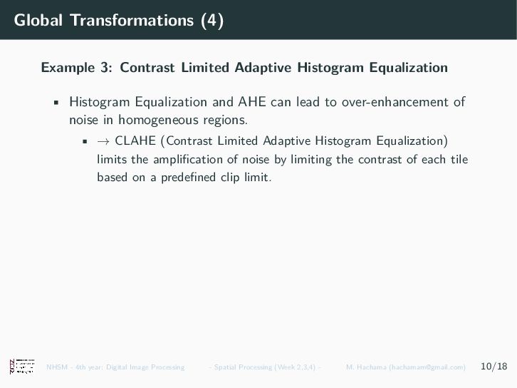
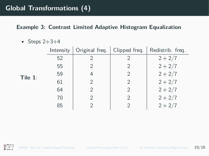
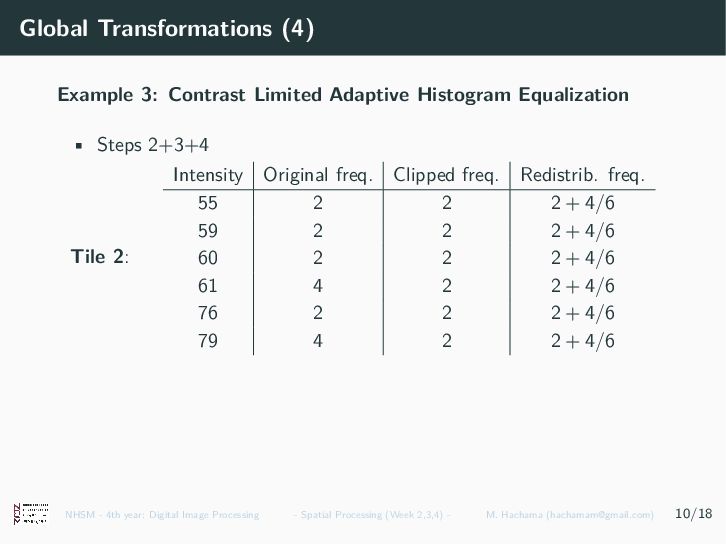
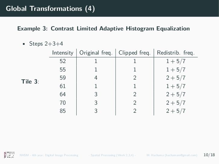
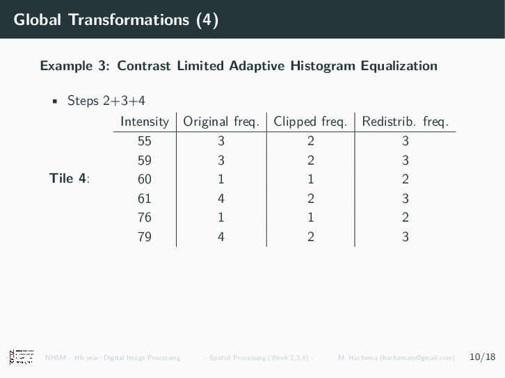
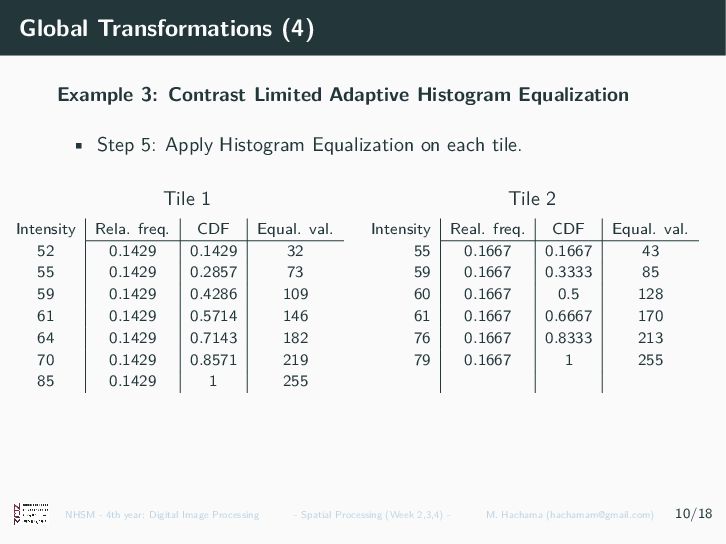
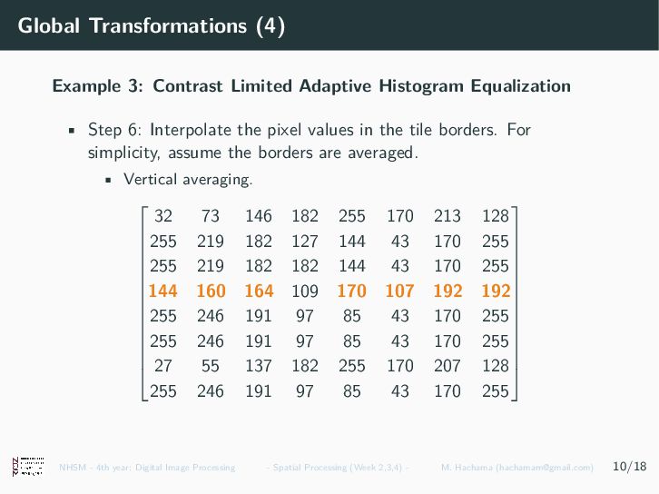
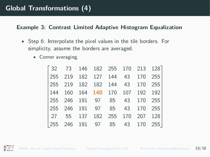
• Histogram Equalization and AHE can lead to over-enhancement of noise in homogeneous regions. • → CLAHE (Contrast Limited Adaptive Histogram Equalization) limits the amplification of noise by limiting the contrast of each tile based on a predefined clip limit. NHSM - 4th year: Digital Image Processing - Spatial Processing (Week 2,3,4) - M. Hachama ([email protected]) 10/18
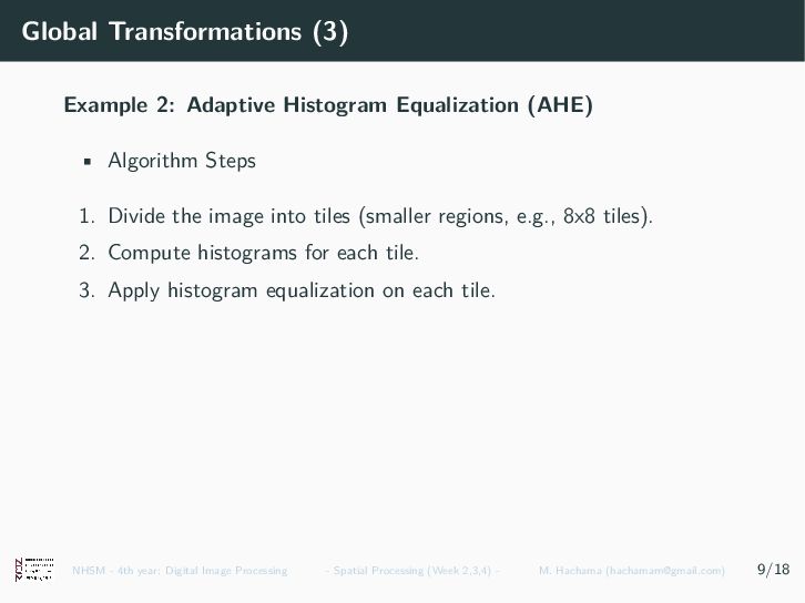
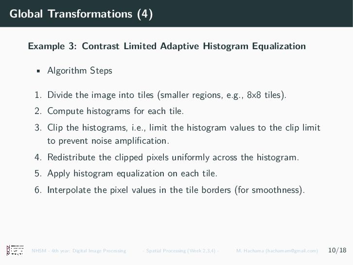
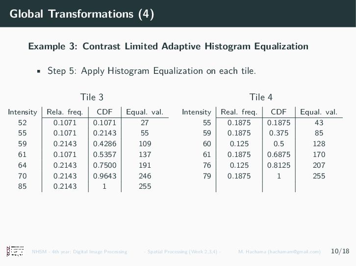
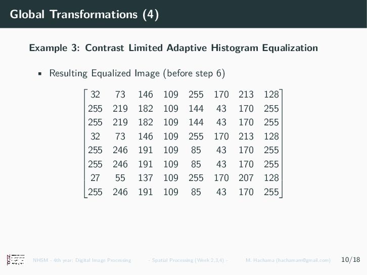
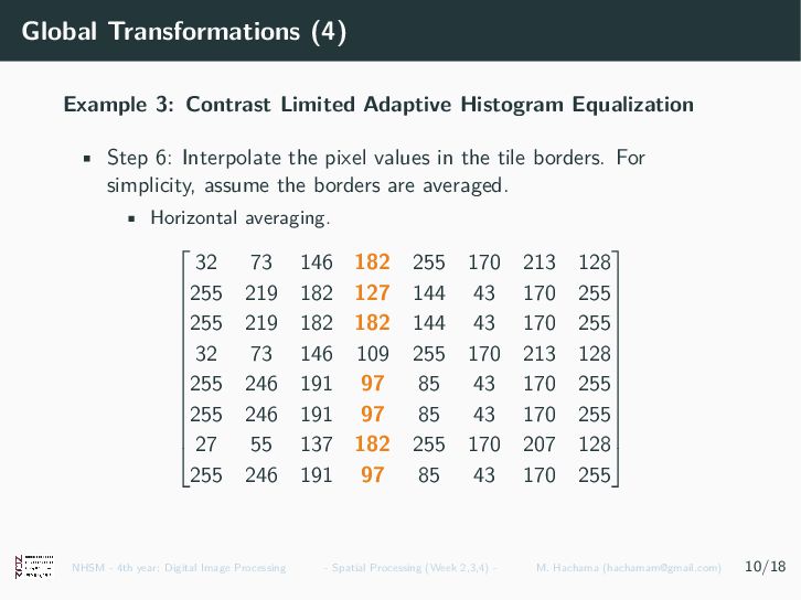
• Algorithm Steps 1. Divide the image into tiles (smaller regions, e.g., 8x8 tiles). 2. Compute histograms for each tile. 3. Clip the histograms, i.e., limit the histogram values to the clip limit to prevent noise amplification. 4. Redistribute the clipped pixels uniformly across the histogram. 5. Apply histogram equalization on each tile. 6. Interpolate the pixel values in the tile borders (for smoothness). NHSM - 4th year: Digital Image Processing - Spatial Processing (Week 2,3,4) - M. Hachama ([email protected]) 10/18
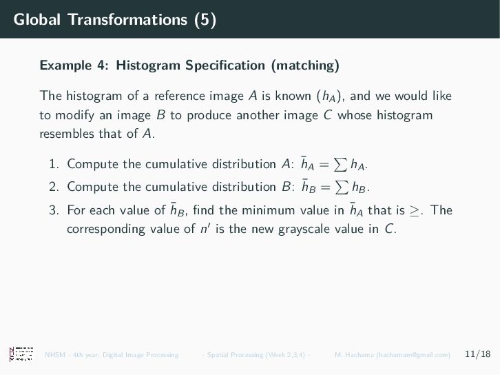
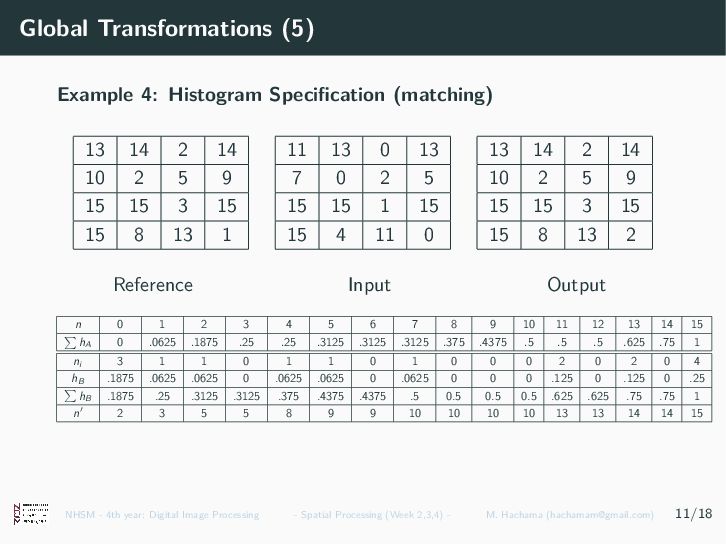
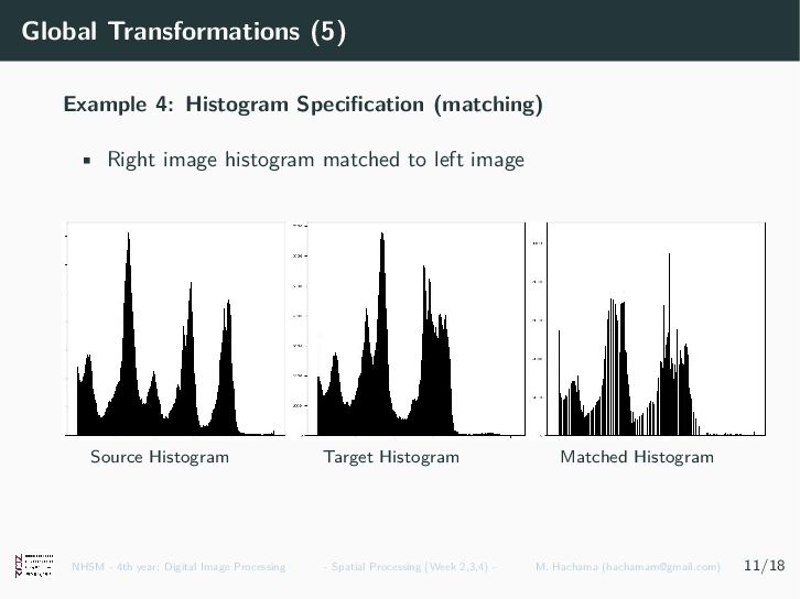
of a reference image A is known (hA ), and we would like to modify an image B to produce another image C whose histogram resembles that of A. 1. Compute the cumulative distribution A: ¯ hA = hA . 2. Compute the cumulative distribution B: ¯ hB = hB . 3. For each value of ¯ hB , find the minimum value in ¯ hA such that ¯ hA ≥ ¯ hB . The corresponding value of n′ is the new grayscale value in C. NHSM - 4th year: Digital Image Processing - Spatial Processing (Week 2,3,4) - M. Hachama ([email protected]) 11/18
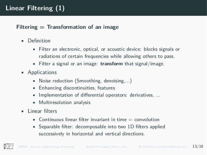
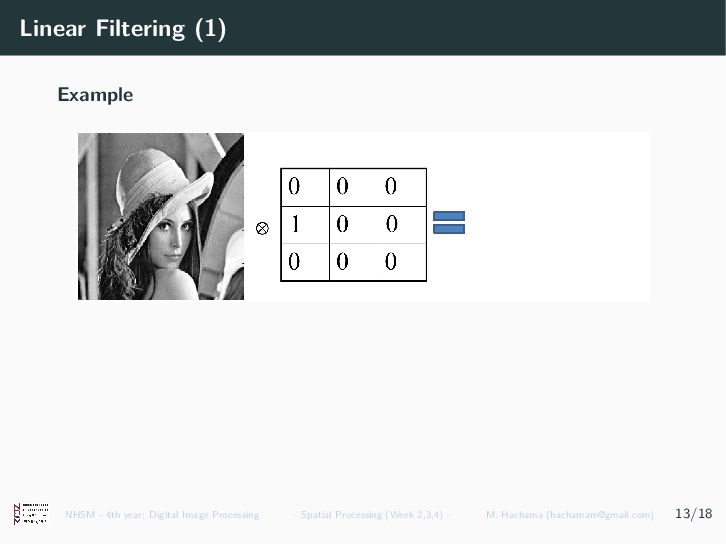
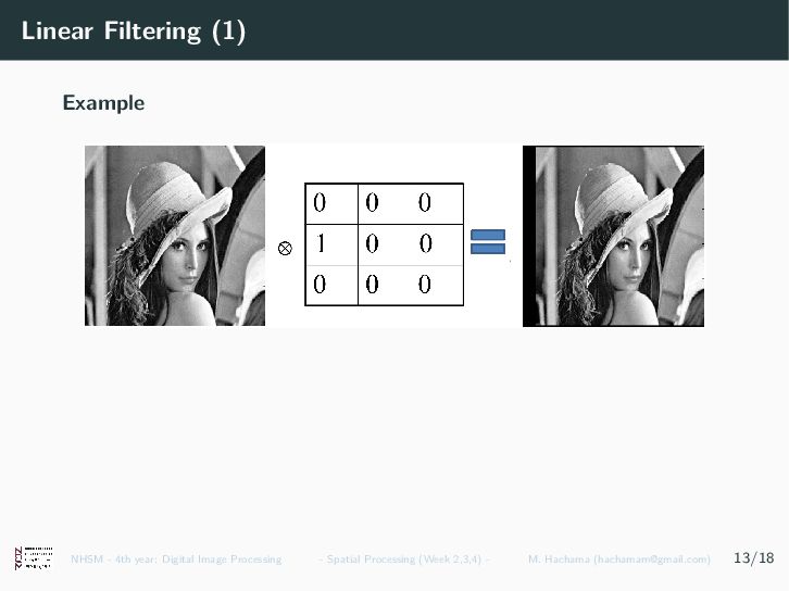
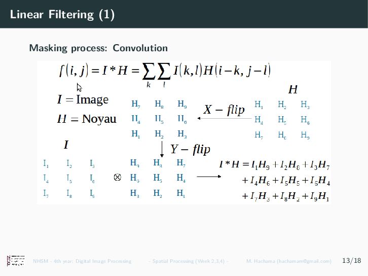
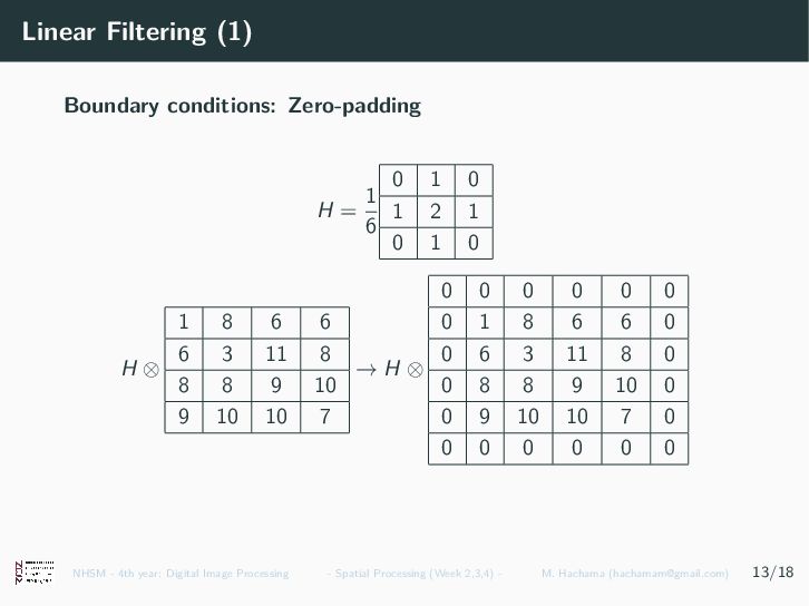
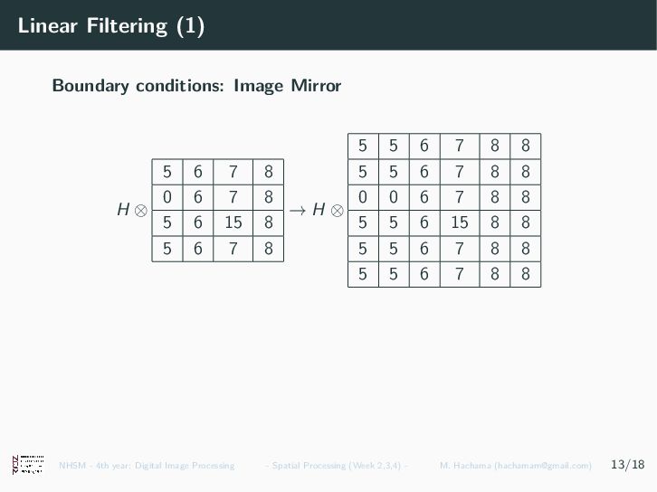
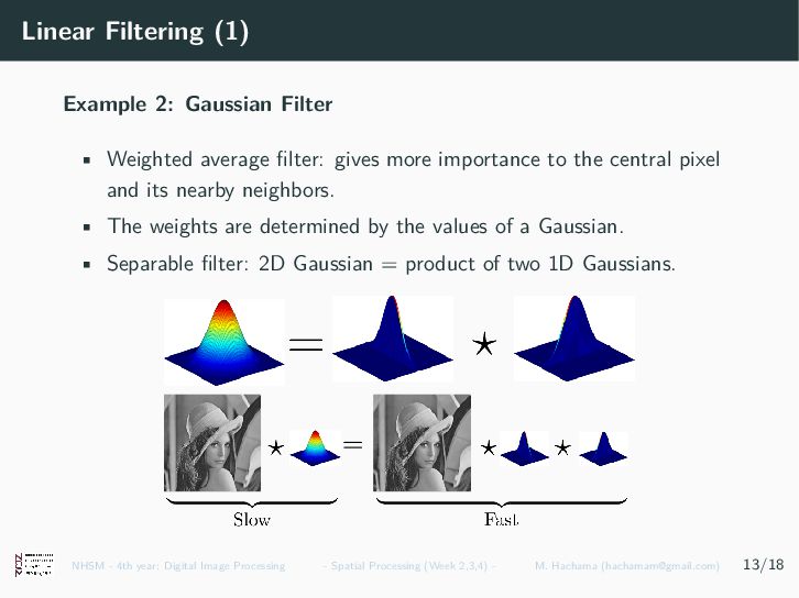
Definition • Filter an electronic, optical, or acoustic device: blocks signals or radiations of certain frequencies while allowing others to pass. • Filter a signal or an image: transform that signal/image. • Applications • Noise reduction (Smoothing, denoising,...) • Enhancing discontinuities, features • Implementation of differential operators: derivatives, ... • Multiresolution analysis • Linear filters • Continuous linear filter invariant in time = convolution • Separable filter: decomposable into two 1D filters applied successively in horizontal and vertical directions. NHSM - 4th year: Digital Image Processing - Spatial Processing (Week 2,3,4) - M. Hachama ([email protected]) 13/18
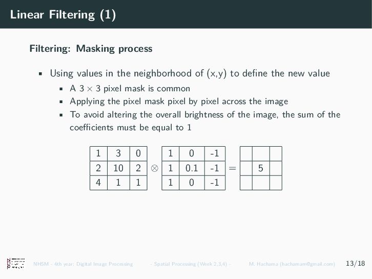
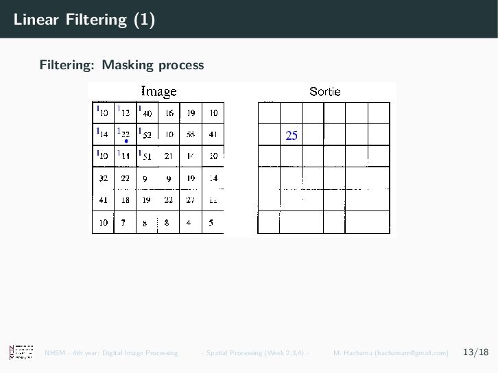
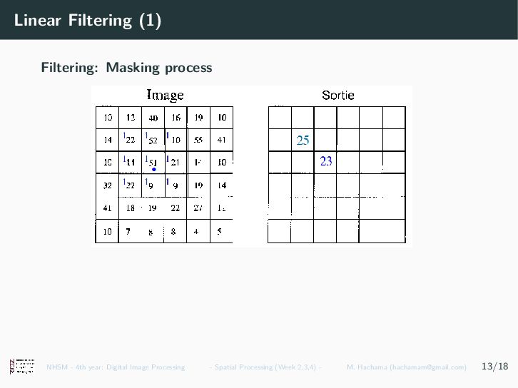
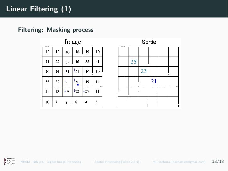
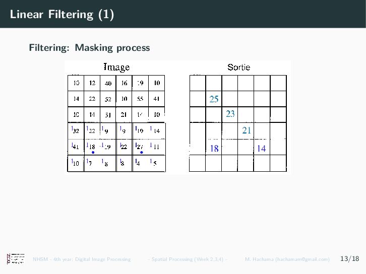
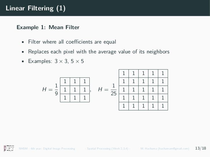
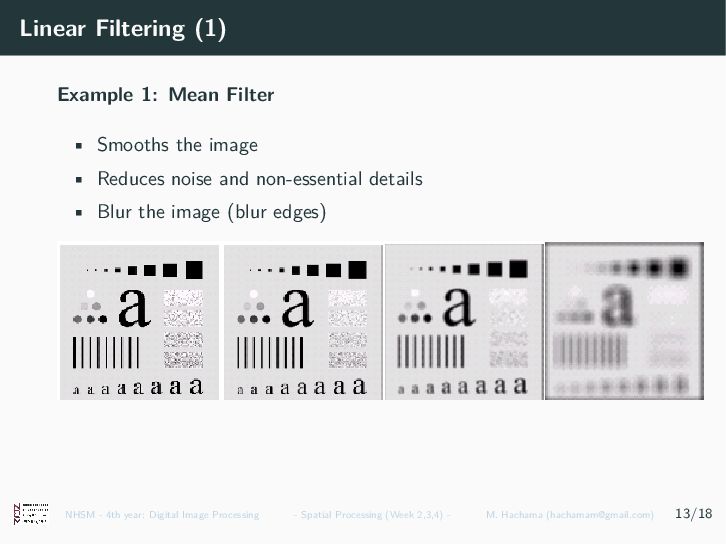
the neighborhood of (x,y) to define the new value • A 3 × 3 pixel mask is common • Applying the pixel mask pixel by pixel across the image • To avoid altering the overall brightness of the image, the sum of the coefficients must be equal to 1 1 3 0 2 10 2 4 1 1 ⊗ 1 0 -1 1 0.1 -1 1 0 -1 = 5 NHSM - 4th year: Digital Image Processing - Spatial Processing (Week 2,3,4) - M. Hachama ([email protected]) 13/18
not process pixels on the edge: Resulting image is smaller! • Partial mask: Process edge pixels with a small number of neighbors. NHSM - 4th year: Digital Image Processing - Spatial Processing (Week 2,3,4) - M. Hachama ([email protected]) 13/18
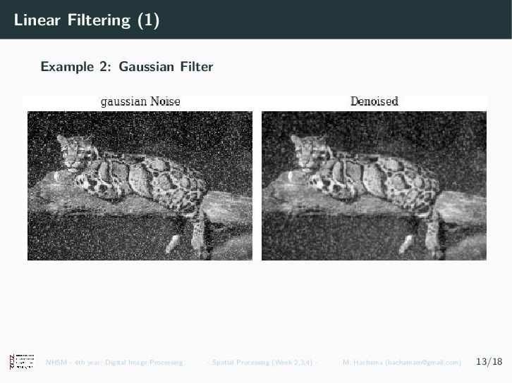
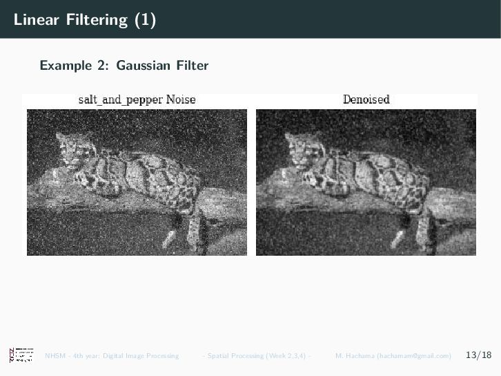
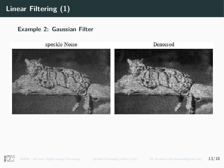
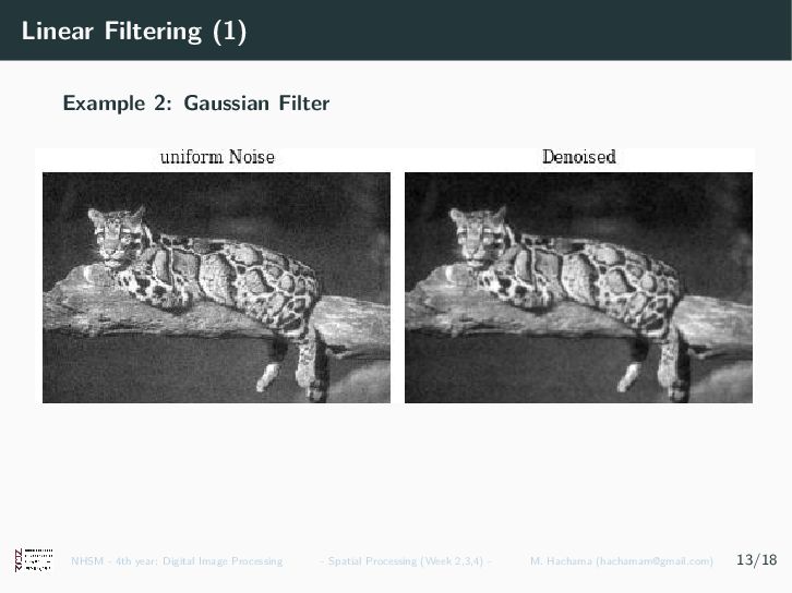
filter: gives more importance to the central pixel and its nearby neighbors. • The weights are determined by the values of a Gaussian. • Separable filter: 2D Gaussian = product of two 1D Gaussians. NHSM - 4th year: Digital Image Processing - Spatial Processing (Week 2,3,4) - M. Hachama ([email protected]) 13/18
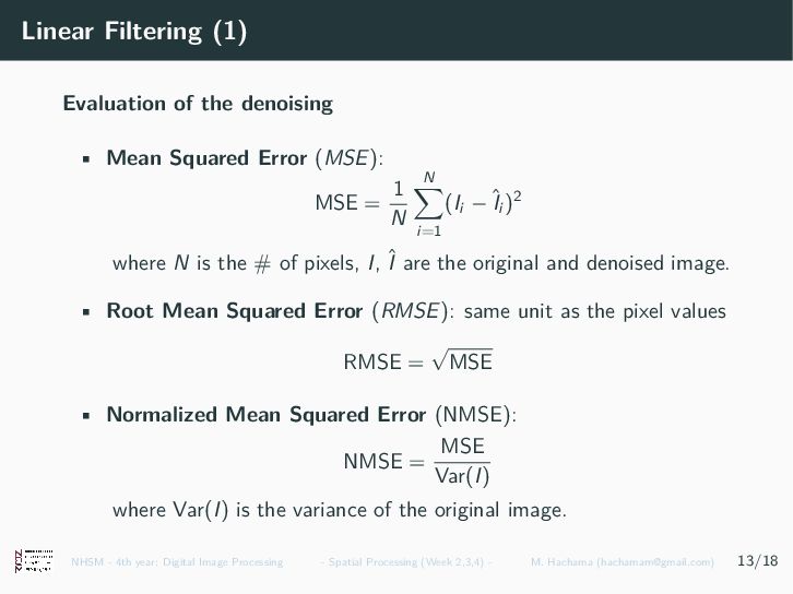
Error (MSE): MSE = 1 N N i=1 (Ii − ˆ Ii )2 where N is the # of pixels, I, ˆ I are the original and denoised image. • Root Mean Squared Error (RMSE): same unit as the pixel values RMSE = √ MSE • Normalized Mean Squared Error (NMSE): NMSE = MSE Var(I) where Var(I) is the variance of the original image. NHSM - 4th year: Digital Image Processing - Spatial Processing (Week 2,3,4) - M. Hachama ([email protected]) 13/18
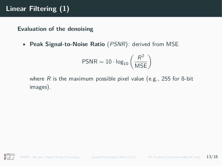
Ratio (PSNR): derived from MSE PSNR = 10 · log 10 R2 MSE where R is the maximum possible pixel value (e.g., 255 for 8-bit images). NHSM - 4th year: Digital Image Processing - Spatial Processing (Week 2,3,4) - M. Hachama ([email protected]) 13/18
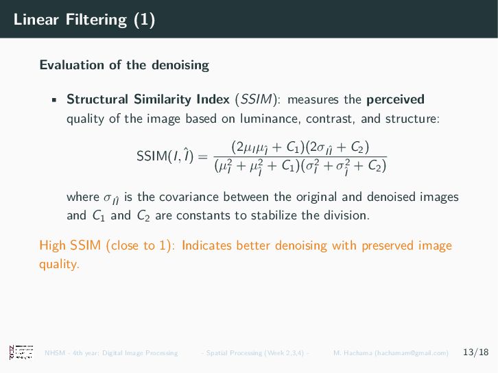
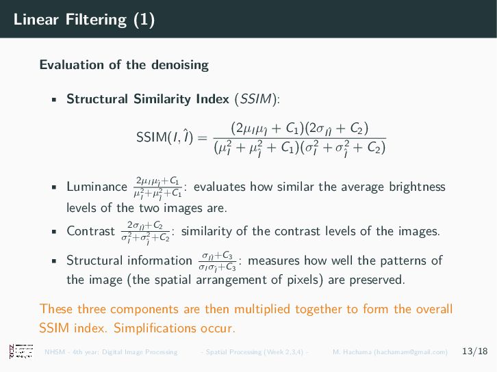
Index (SSIM): SSIM(I,ˆ I) = (2µI µˆ I + C1 )(2σ Iˆ I + C2 ) (µ2 I + µ2 ˆ I + C1 )(σ2 I + σ2 ˆ I + C2 ) where µ and σ are the mean and variance/covariance values. C1 and C2 are constants to stabilize the division. • Luminance 2µI µˆ I +C1 µ2 I +µ2 ˆ I +C1 = Similarity of the average brightness. • Contrast 2σ Iˆ I +C2 σ2 I +σ2 ˆ I +C2 : Covariance based criterion. High SSIM (∼ 1) indicates better denoising with preserved image quality. NHSM - 4th year: Digital Image Processing - Spatial Processing (Week 2,3,4) - M. Hachama ([email protected]) 13/18
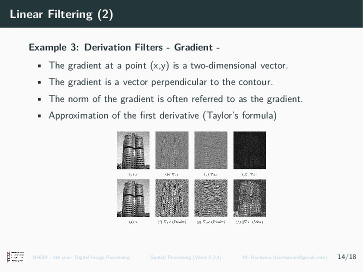
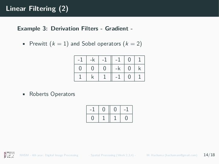
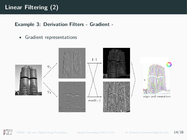
• The gradient at a point (x,y) is a two-dimensional vector. • The gradient is a vector perpendicular to the contour. • The norm of the gradient is often referred to as the gradient. • Approximation of the first derivative (Taylor’s formula) NHSM - 4th year: Digital Image Processing - Spatial Processing (Week 2,3,4) - M. Hachama ([email protected]) 14/18
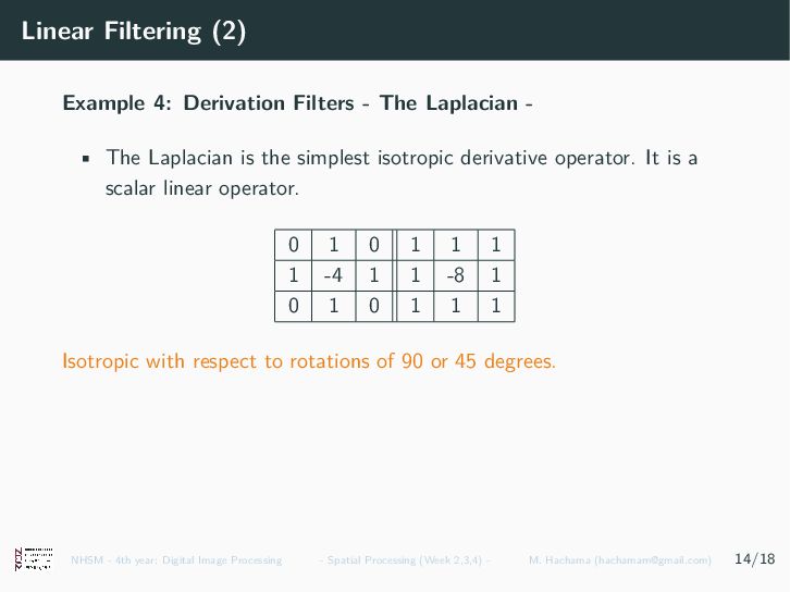
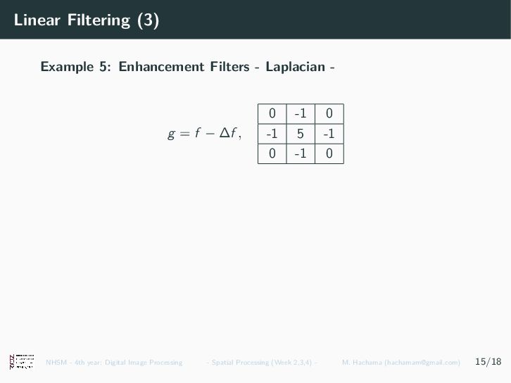
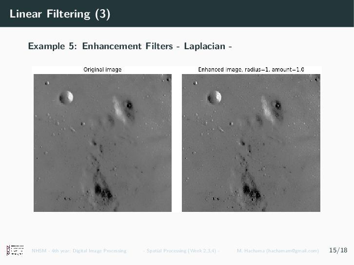
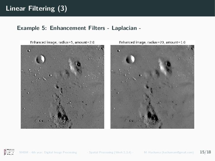
- • The Laplacian is the simplest isotropic derivative operator. It is a scalar linear operator. 0 1 0 1 1 1 1 -4 1 1 -8 1 0 1 0 1 1 1 Isotropic with respect to rotations of 90 or 45 degrees. NHSM - 4th year: Digital Image Processing - Spatial Processing (Week 2,3,4) - M. Hachama ([email protected]) 14/18
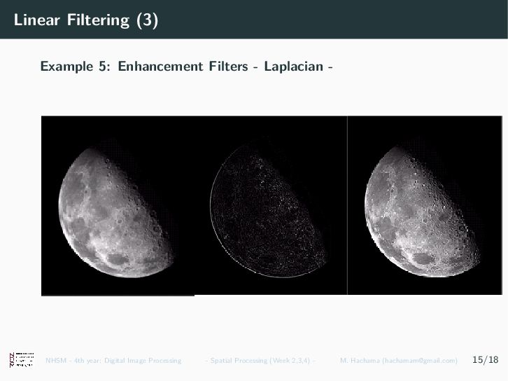
g = f + λ(f − fb ) where fb is a regularized version (median, gaussian, ...) NHSM - 4th year: Digital Image Processing - Spatial Processing (Week 2,3,4) - M. Hachama ([email protected]) 15/18
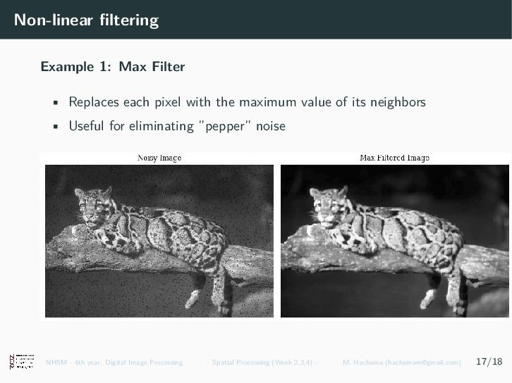
value selected based on a criterion, e.g., statistical • Cannot be implemented as a convolution product • Reduces noise with less blurring NHSM - 4th year: Digital Image Processing - Spatial Processing (Week 2,3,4) - M. Hachama ([email protected]) 17/18
with the maximum value of its neighbors • Useful for eliminating ”pepper” noise NHSM - 4th year: Digital Image Processing - Spatial Processing (Week 2,3,4) - M. Hachama ([email protected]) 17/18
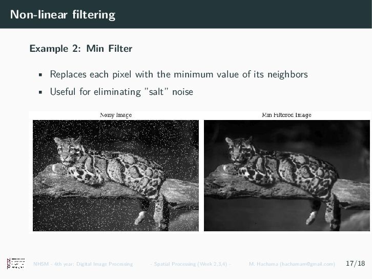
with the minimum value of its neighbors • Useful for eliminating ”salt” noise NHSM - 4th year: Digital Image Processing - Spatial Processing (Week 2,3,4) - M. Hachama ([email protected]) 17/18
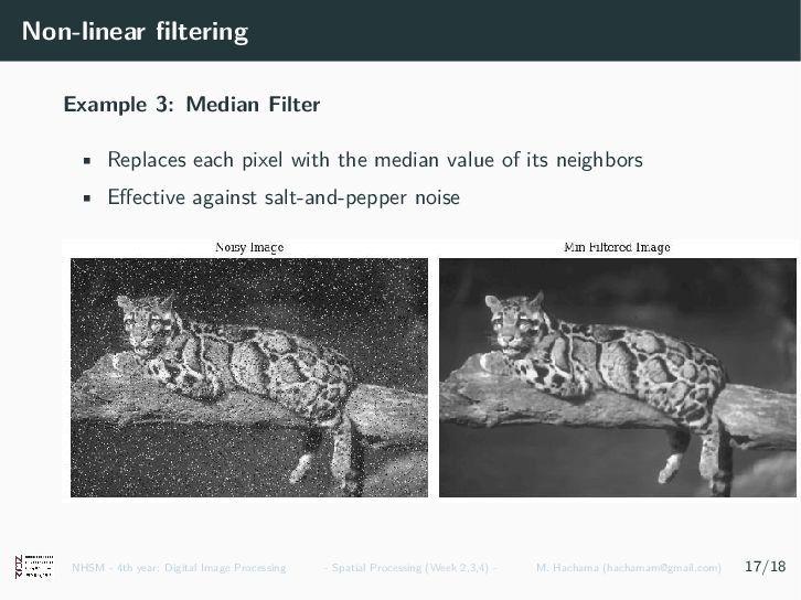
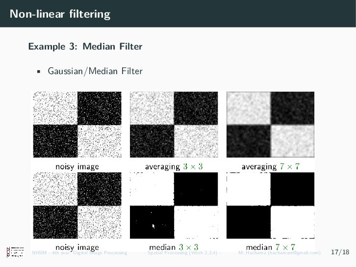
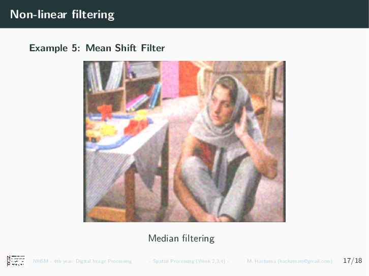
with the median value of its neighbors • Effective against salt-and-pepper noise NHSM - 4th year: Digital Image Processing - Spatial Processing (Week 2,3,4) - M. Hachama ([email protected]) 17/18
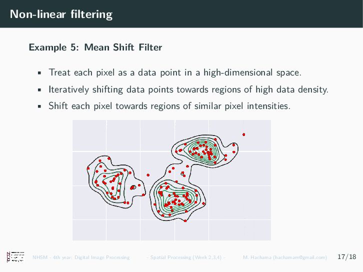
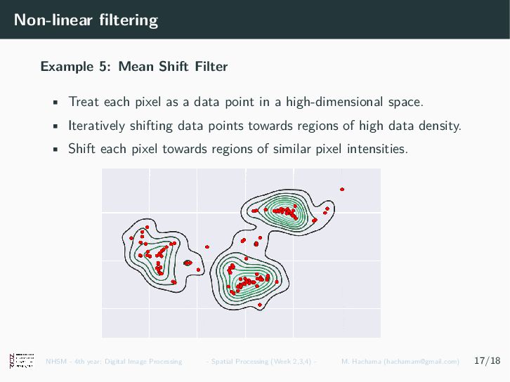
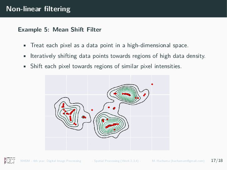
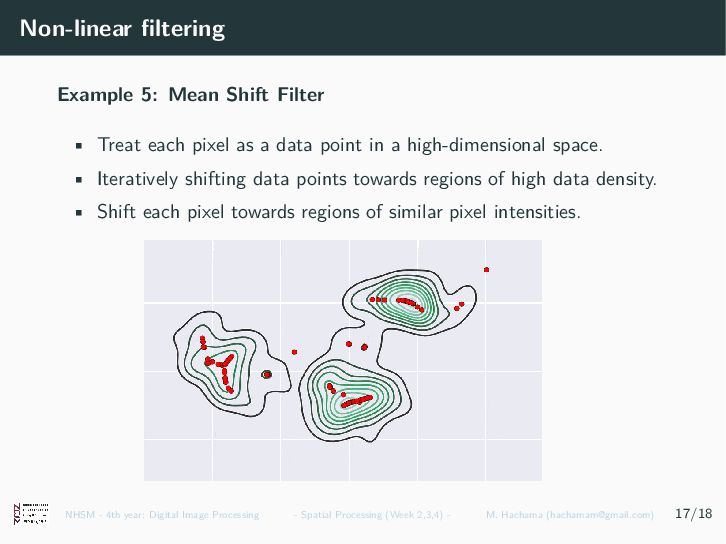
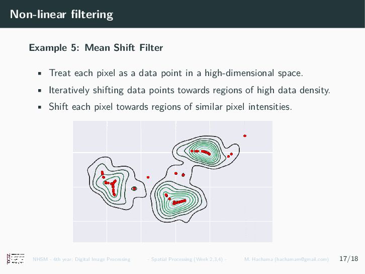
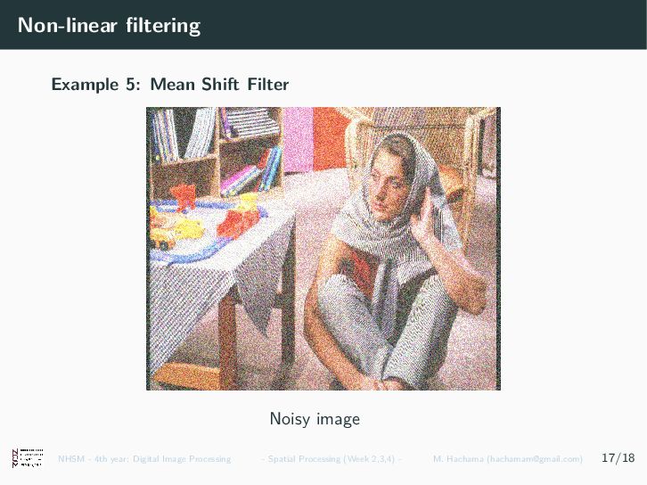
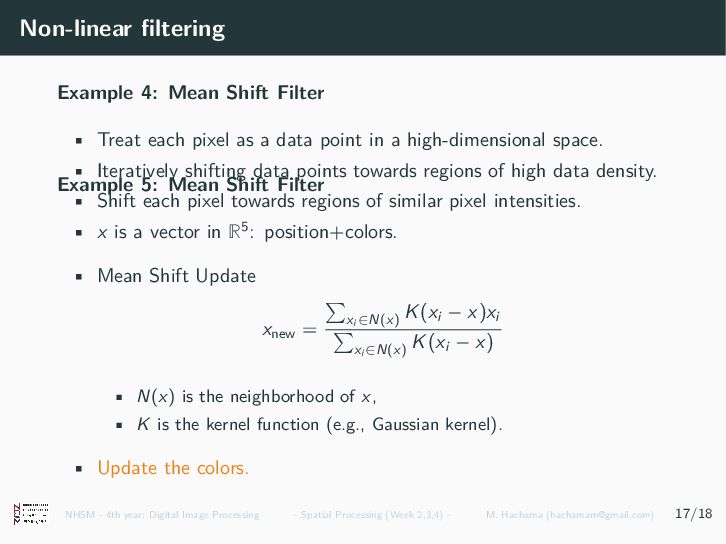
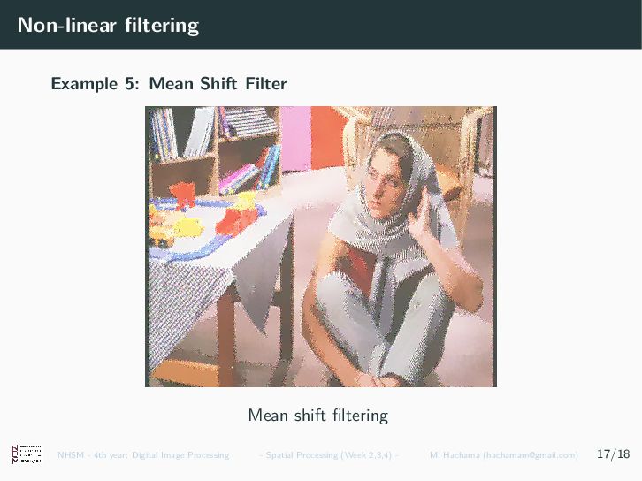
pixel as a data point in a high-dimensional space. • Iteratively shifting data points towards regions of high data density. • Shift each pixel towards regions of similar pixel intensities. NHSM - 4th year: Digital Image Processing - Spatial Processing (Week 2,3,4) - M. Hachama ([email protected]) 17/18
pixel as a data point in a high-dimensional space. • Iteratively shifting data points towards regions of high data density. • Shift each pixel towards regions of similar pixel intensities. NHSM - 4th year: Digital Image Processing - Spatial Processing (Week 2,3,4) - M. Hachama ([email protected]) 17/18
pixel as a data point in a high-dimensional space. • Iteratively shifting data points towards regions of high data density. • Shift each pixel towards regions of similar pixel intensities. NHSM - 4th year: Digital Image Processing - Spatial Processing (Week 2,3,4) - M. Hachama ([email protected]) 17/18
pixel as a data point in a high-dimensional space. • Iteratively shifting data points towards regions of high data density. • Shift each pixel towards regions of similar pixel intensities. NHSM - 4th year: Digital Image Processing - Spatial Processing (Week 2,3,4) - M. Hachama ([email protected]) 17/18
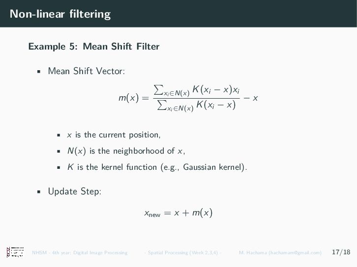
pixel as a data point in a high-dimensional space. • Iteratively shifting data points towards regions of high data density. • Shift each pixel towards regions of similar pixel intensities. Example 5: Mean Shift Filter • x is a vector in R5: position+colors. • Mean Shift Update xnew = xi ∈N(x) K(xi − x)xi xi ∈N(x) K(xi − x) • N(x) is the neighborhood of x, • K is the kernel function (e.g., Gaussian kernel). • Update the colors. NHSM - 4th year: Digital Image Processing - Spatial Processing (Week 2,3,4) - M. Hachama ([email protected]) 17/18
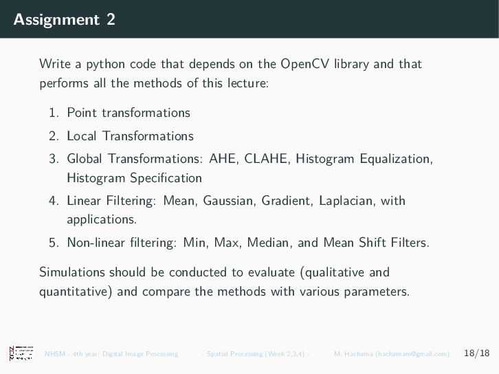
OpenCV library and that performs all the methods of this lecture: 1. Point transformations 2. Local Transformations 3. Global Transformations: AHE, CLAHE, Histogram Equalization, Histogram Specification 4. Linear Filtering: Mean, Gaussian, Gradient, Laplacian, with applications. 5. Non-linear filtering: Min, Max, Median, and Mean Shift Filters. Simulations should be conducted to evaluate (qualitative and quantitative) and compare the methods with various parameters. NHSM - 4th year: Digital Image Processing - Spatial Processing (Week 2,3,4) - M. Hachama ([email protected]) 18/18