SPICE Modeling and Device Modeling of Solar Cells: From Device Physics to Parameter Extraction, SPICE Implementation, and Validation (Graduate Lecture Notes)

These graduate-level lecture notes provide a comprehensive guide to solar cell and module SPICE modeling. They cover the role of compact modeling, semiconductor device physics (photogeneration, recombination mechanisms, superposition), equivalent-circuit models (single-diode, double-diode, and Bishop reverse-bias models), implicit equation solvers (Lambert W function and numerical methods), and parameter extraction techniques such as the De Soto method. Furthermore, the notes explain temperature and irradiance scaling, module/array scaling, partial shading and bypass diodes, SPICE implementation (behavioral and Verilog-A approaches), validation frameworks, and extensions to emerging technologies like high-efficiency silicon and perovskite/silicon tandems.

Transcript

1. SPICE Modeling and Device Modeling of Solar Cells From device physics to equivalent circuits, parameter extraction, SPICE implementation and validation (graduate lecture notes) Bee Technologies Inc. November 2026
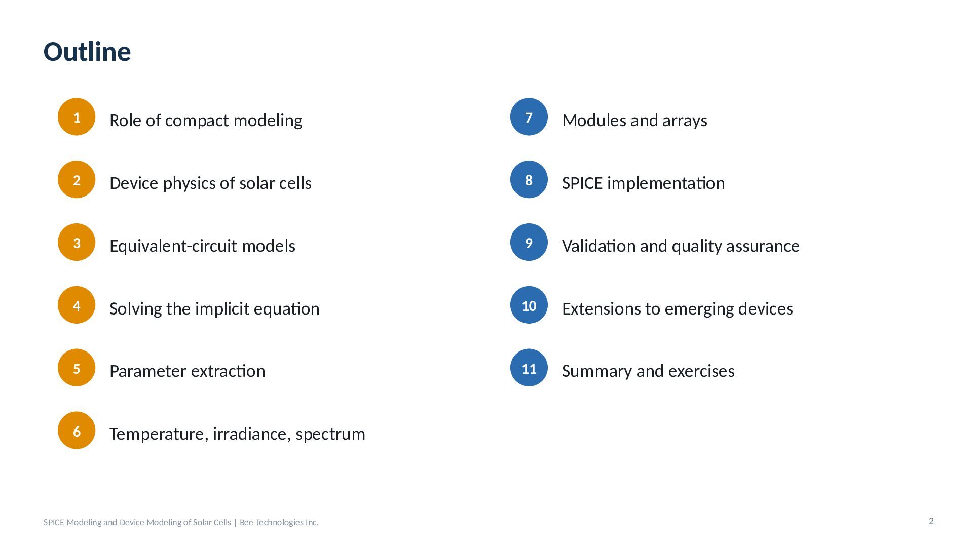
2. Outline 1 Role of compact modeling 7 Modules and arrays 2 Device physics of solar cells 8 SPICE implementation 3 Equivalent-circuit models 9 Validation and quality assurance 4 Solving the implicit equation 10 Extensions to emerging devices 5 Parameter extraction 11 Summary and exercises 6 Temperature, irradiance, spectrum SPICE Modeling and Device Modeling of Solar Cells | Bee Technologies Inc. 2
3. 01 Role of Compact Modeling Why solar cells need SPICE models, and at which level of abstraction 3
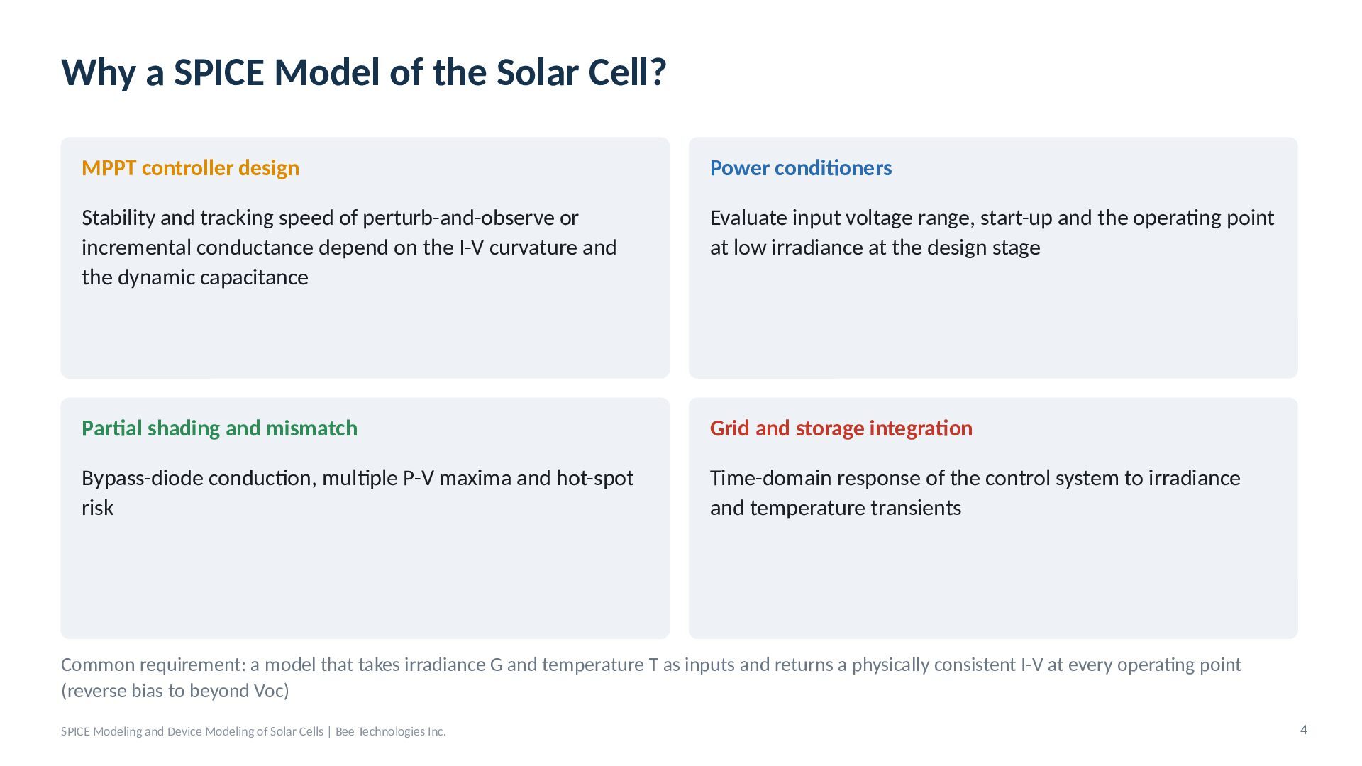
4. Why a SPICE Model of the Solar Cell? MPPT controller design Power conditioners Stability and tracking speed of perturb-and-observe or incremental conductance depend on the I-V curvature and the dynamic capacitance Evaluate input voltage range, start-up and the operating point at low irradiance at the design stage Partial shading and mismatch Grid and storage integration Bypass-diode conduction, multiple P-V maxima and hot-spot risk Time-domain response of the control system to irradiance and temperature transients Common requirement: a model that takes irradiance G and temperature T as inputs and returns a physically consistent I-V at every operating point (reverse bias to beyond Voc) SPICE Modeling and Device Modeling of Solar Cells | Bee Technologies Inc. 4
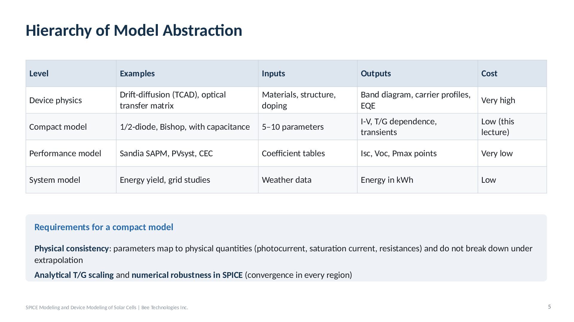
5. Hierarchy of Model Abstraction Level Examples Inputs Outputs Cost Device physics Drift-diffusion (TCAD), optical transfer matrix Materials, structure, doping Band diagram, carrier profiles, EQE Very high Compact model 1/2-diode, Bishop, with capacitance 5–10 parameters I-V, T/G dependence, transients Low (this lecture) Performance model Sandia SAPM, PVsyst, CEC Coefficient tables Isc, Voc, Pmax points Very low System model Energy yield, grid studies Weather data Energy in kWh Low Requirements for a compact model Physical consistency: parameters map to physical quantities (photocurrent, saturation current, resistances) and do not break down under extrapolation Analytical T/G scaling and numerical robustness in SPICE (convergence in every region) SPICE Modeling and Device Modeling of Solar Cells | Bee Technologies Inc. 5
6. 02 Device Physics of Solar Cells Photogeneration, dark current, recombination, figures of merit 6
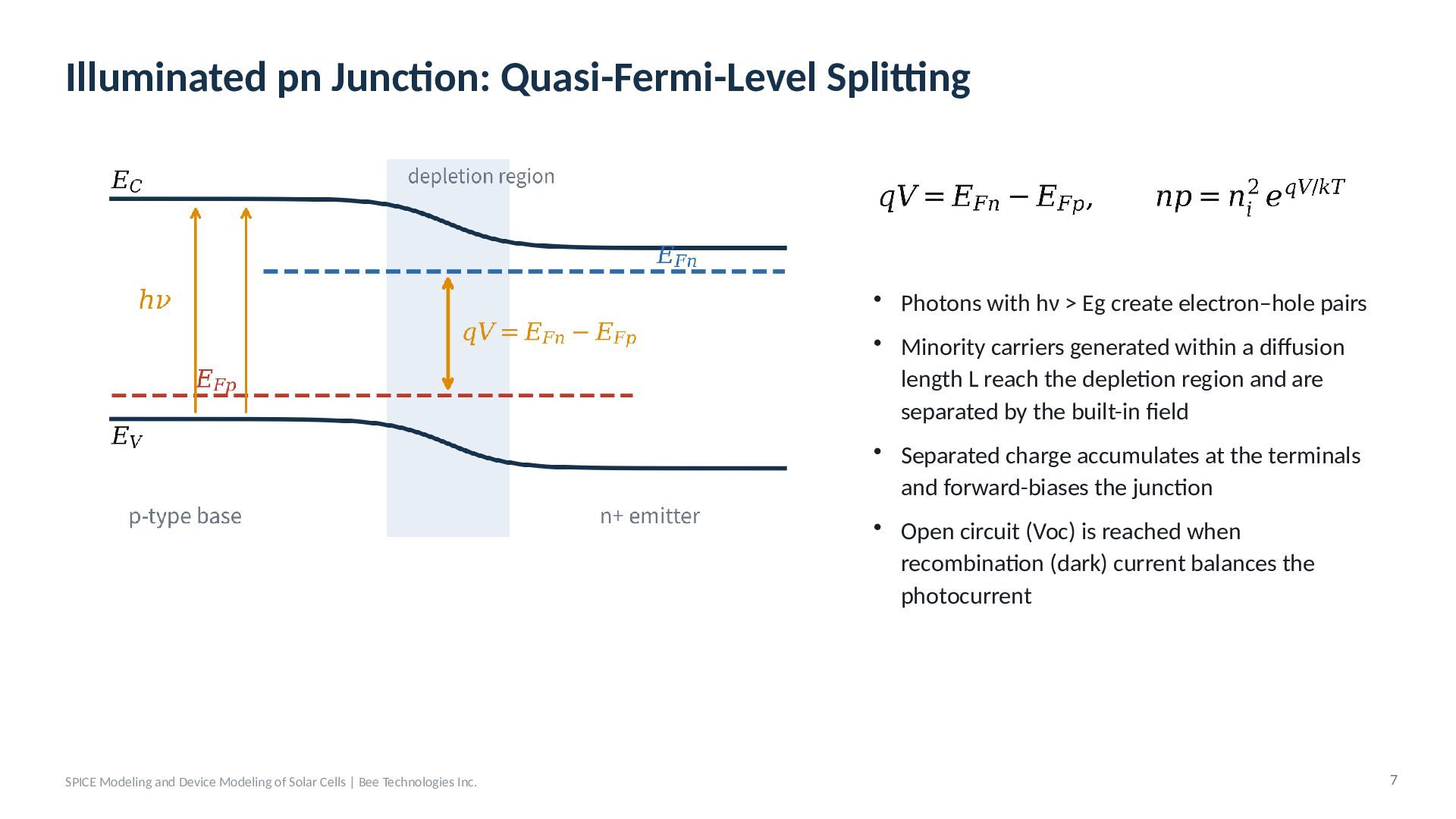
7. Illuminated pn Junction: Quasi-Fermi-Level Splitting • Photons with hν > Eg create electron–hole pairs • Minority carriers generated within a diffusion length L reach the depletion region and are separated by the built-in field • Separated charge accumulates at the terminals and forward-biases the junction • Open circuit (Voc) is reached when recombination (dark) current balances the photocurrent SPICE Modeling and Device Modeling of Solar Cells | Bee Technologies Inc. 7
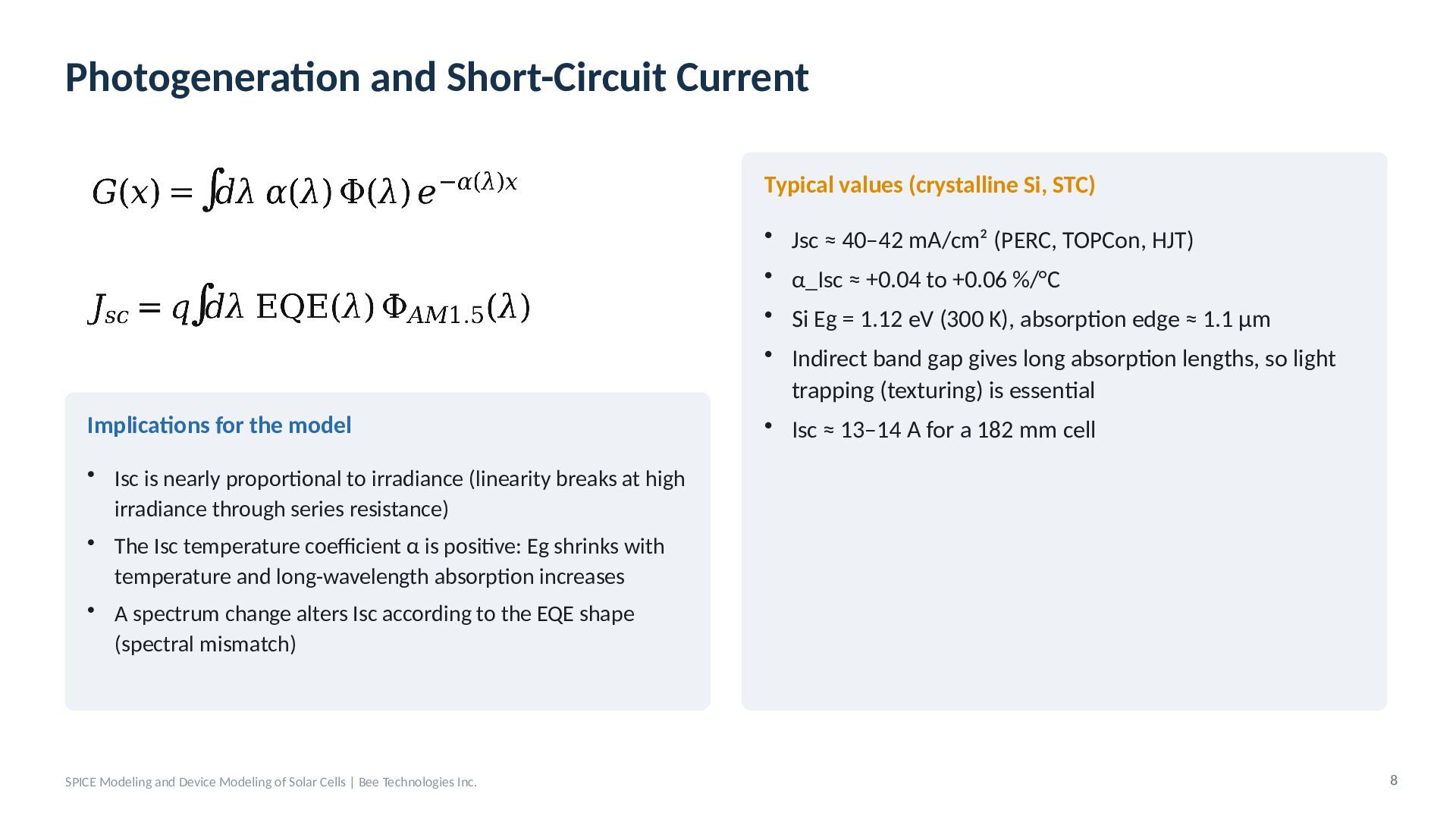
8. Photogeneration and Short-Circuit Current Typical values (crystalline Si, STC) • Jsc ≈ 40–42 mA/cm² (PERC, TOPCon, HJT) • α_Isc ≈ +0.04 to +0.06 %/°C Implications for the model • Si Eg = 1.12 eV (300 K), absorption edge ≈ 1.1 µm • Indirect band gap gives long absorption lengths, so light trapping (texturing) is essential • Isc ≈ 13–14 A for a 182 mm cell • Isc is nearly proportional to irradiance (linearity breaks at high irradiance through series resistance) • The Isc temperature coefficient α is positive: Eg shrinks with temperature and long-wavelength absorption increases • A spectrum change alters Isc according to the EQE shape (spectral mismatch) SPICE Modeling and Device Modeling of Solar Cells | Bee Technologies Inc. 8
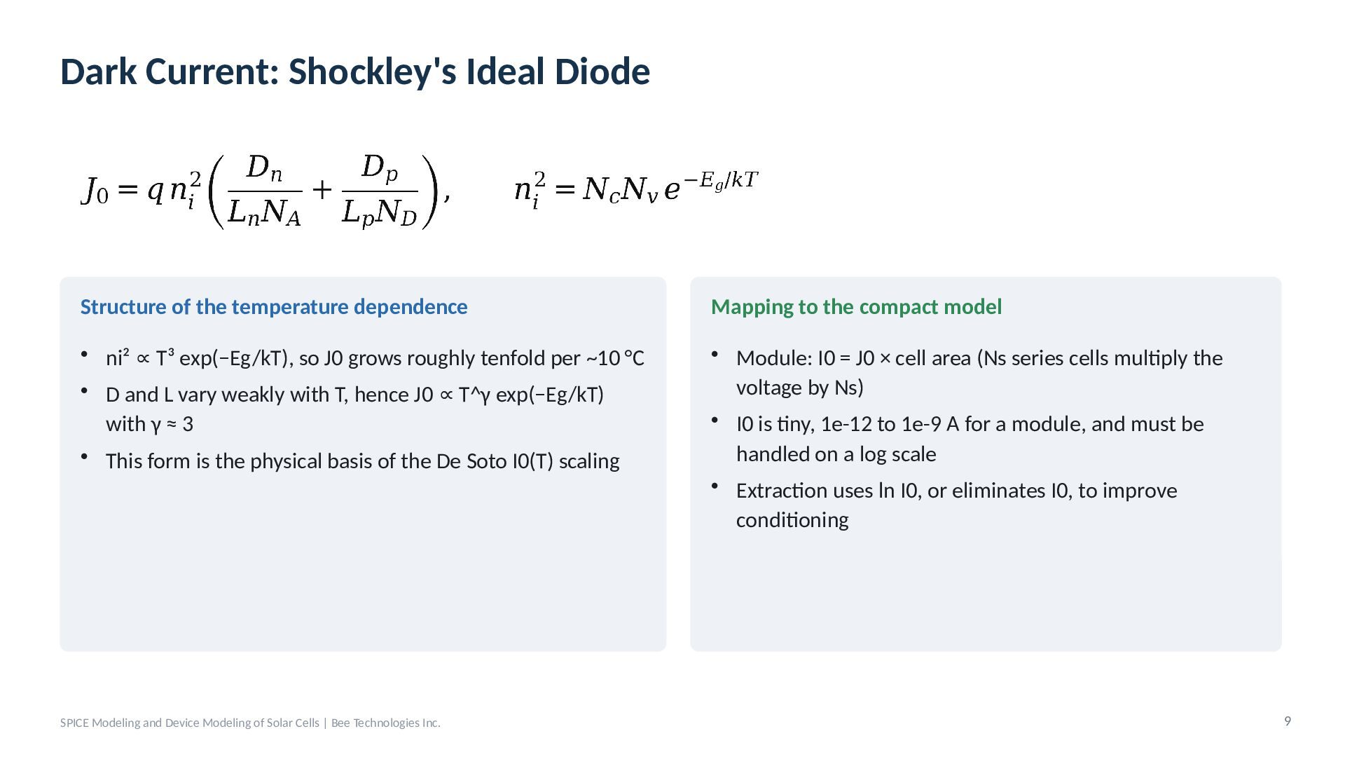
9. Dark Current: Shockley's Ideal Diode Structure of the temperature dependence Mapping to the compact model • ni² ∝ T³ exp(−Eg/kT), so J0 grows roughly tenfold per ~10 °C • D and L vary weakly with T, hence J0 ∝ T^γ exp(−Eg/kT) with γ ≈ 3 • This form is the physical basis of the De Soto I0(T) scaling • Module: I0 = J0 × cell area (Ns series cells multiply the voltage by Ns) • I0 is tiny, 1e-12 to 1e-9 A for a module, and must be handled on a log scale • Extraction uses ln I0, or eliminates I0, to improve conditioning SPICE Modeling and Device Modeling of Solar Cells | Bee Technologies Inc. 9
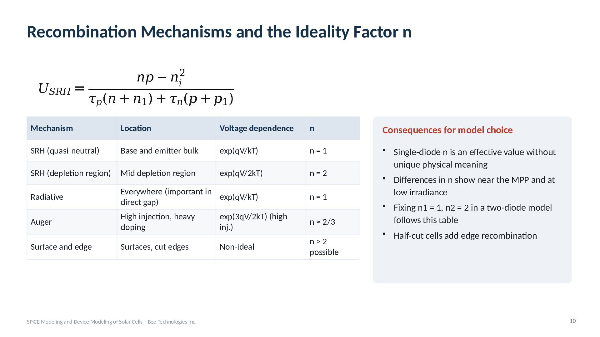
10. Recombination Mechanisms and the Ideality Factor n Mechanism Location Voltage dependence n Consequences for model choice SRH (quasi-neutral) Base and emitter bulk exp(qV/kT) n=1 SRH (depletion region) Mid depletion region exp(qV/2kT) n=2 Radiative Everywhere (important in exp(qV/kT) direct gap) n=1 Auger High injection, heavy doping exp(3qV/2kT) (high inj.) n ≈ 2/3 Surface and edge Surfaces, cut edges Non-ideal n>2 possible • Single-diode n is an effective value without unique physical meaning • Differences in n show near the MPP and at low irradiance • Fixing n1 = 1, n2 = 2 in a two-diode model follows this table • Half-cut cells add edge recombination SPICE Modeling and Device Modeling of Solar Cells | Bee Technologies Inc. 10
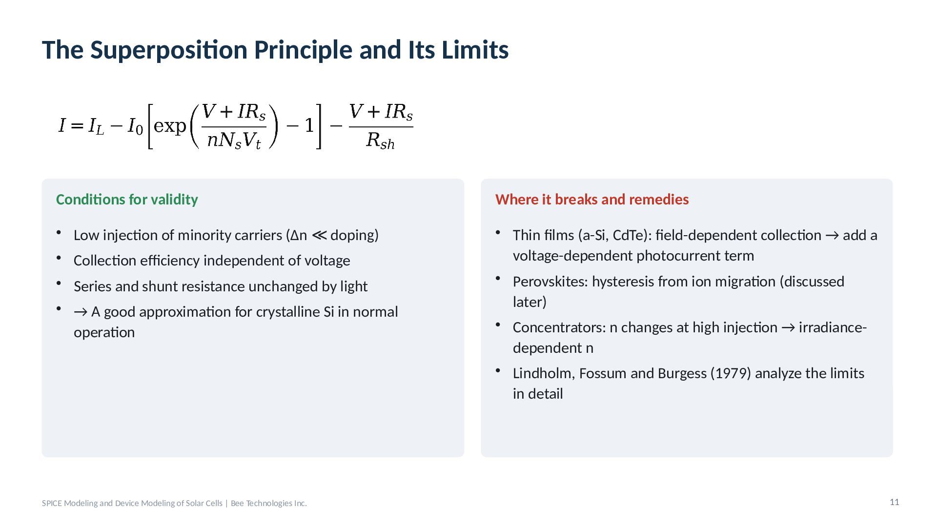
11. The Superposition Principle and Its Limits Conditions for validity Where it breaks and remedies • Low injection of minority carriers (Δn ≪ doping) • Collection efficiency independent of voltage • Thin films (a-Si, CdTe): field-dependent collection → add a voltage-dependent photocurrent term • Perovskites: hysteresis from ion migration (discussed later) • Concentrators: n changes at high injection → irradiancedependent n • Lindholm, Fossum and Burgess (1979) analyze the limits in detail • Series and shunt resistance unchanged by light • → A good approximation for crystalline Si in normal operation SPICE Modeling and Device Modeling of Solar Cells | Bee Technologies Inc. 11
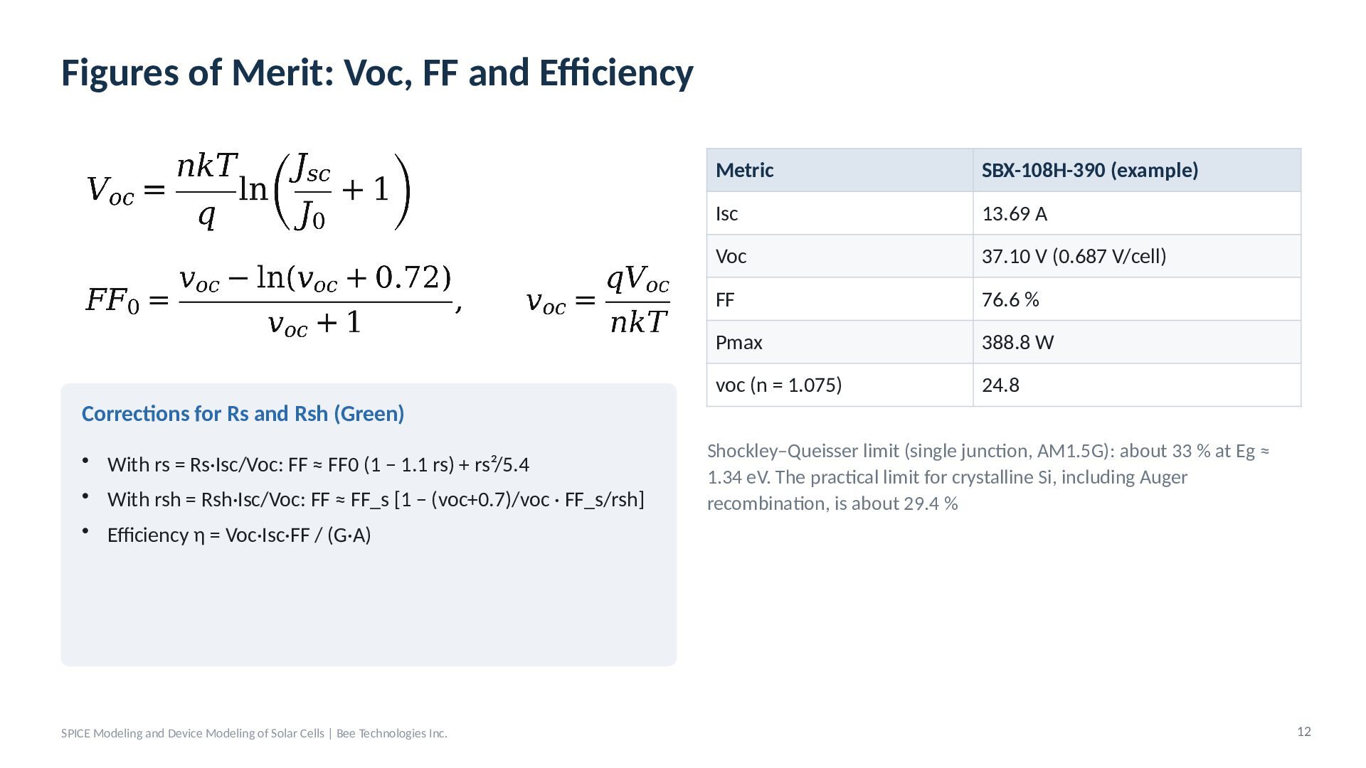
12. Figures of Merit: Voc, FF and Efficiency Metric SBX-108H-390 (example) Isc 13.69 A Voc 37.10 V (0.687 V/cell) FF 76.6 % Pmax 388.8 W voc (n = 1.075) 24.8 Corrections for Rs and Rsh (Green) • With rs = Rs·Isc/Voc: FF ≈ FF0 (1 − 1.1 rs) + rs²/5.4 • With rsh = Rsh·Isc/Voc: FF ≈ FF_s [1 − (voc+0.7)/voc · FF_s/rsh] Shockley–Queisser limit (single junction, AM1.5G): about 33 % at Eg ≈ 1.34 eV. The practical limit for crystalline Si, including Auger recombination, is about 29.4 % • Efficiency η = Voc·Isc·FF / (G·A) SPICE Modeling and Device Modeling of Solar Cells | Bee Technologies Inc. 12
13. 03 Equivalent-Circuit Models Single diode, double diode, reverse bias, dynamic models, emerging devices 13
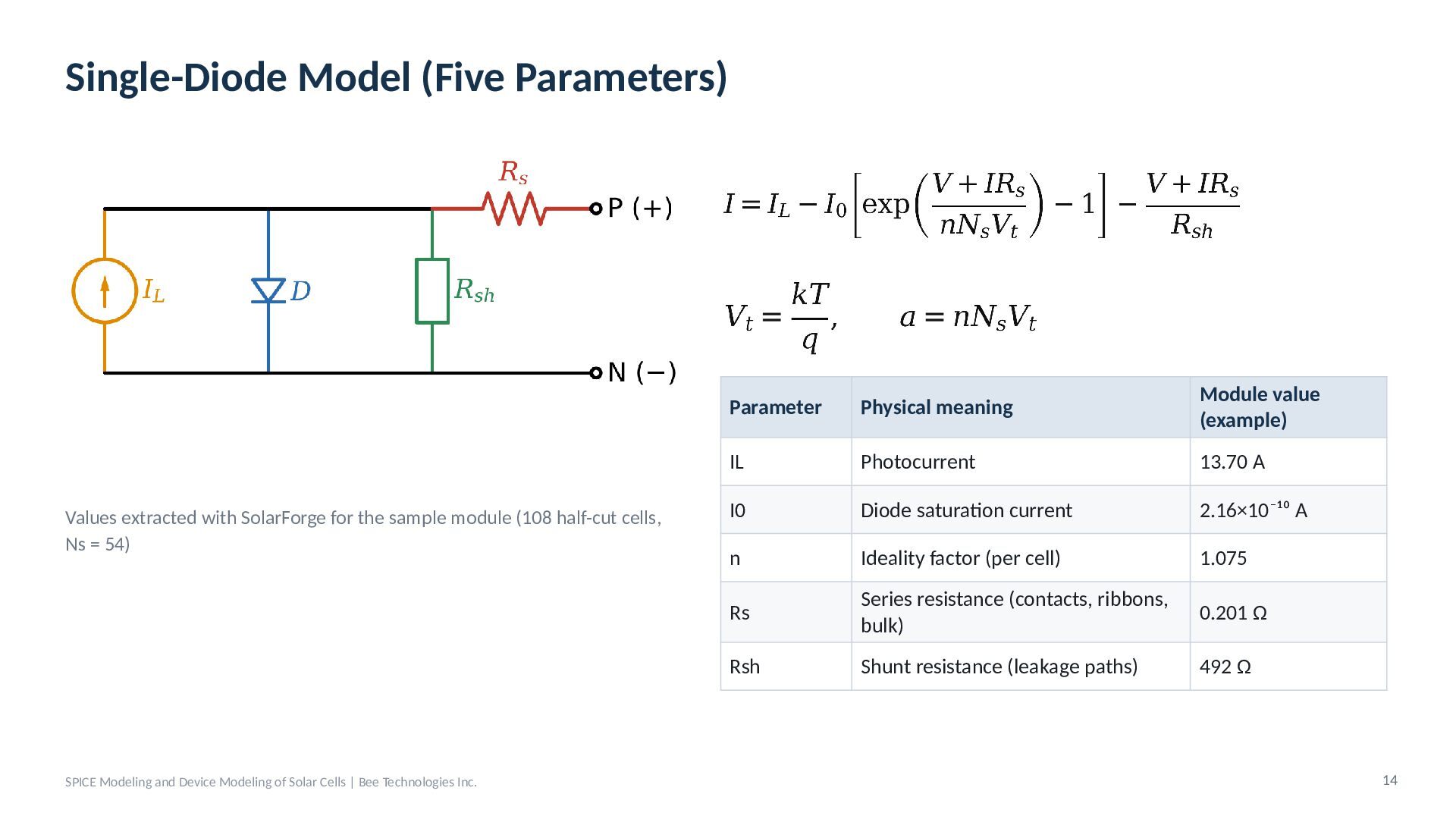
14. Single-Diode Model (Five Parameters) Values extracted with SolarForge for the sample module (108 half-cut cells, Ns = 54) SPICE Modeling and Device Modeling of Solar Cells | Bee Technologies Inc. Parameter Physical meaning Module value (example) IL Photocurrent 13.70 A I0 Diode saturation current 2.16×10⁻¹⁰ A n Ideality factor (per cell) 1.075 Rs Series resistance (contacts, ribbons, bulk) 0.201 Ω Rsh Shunt resistance (leakage paths) 492 Ω 14
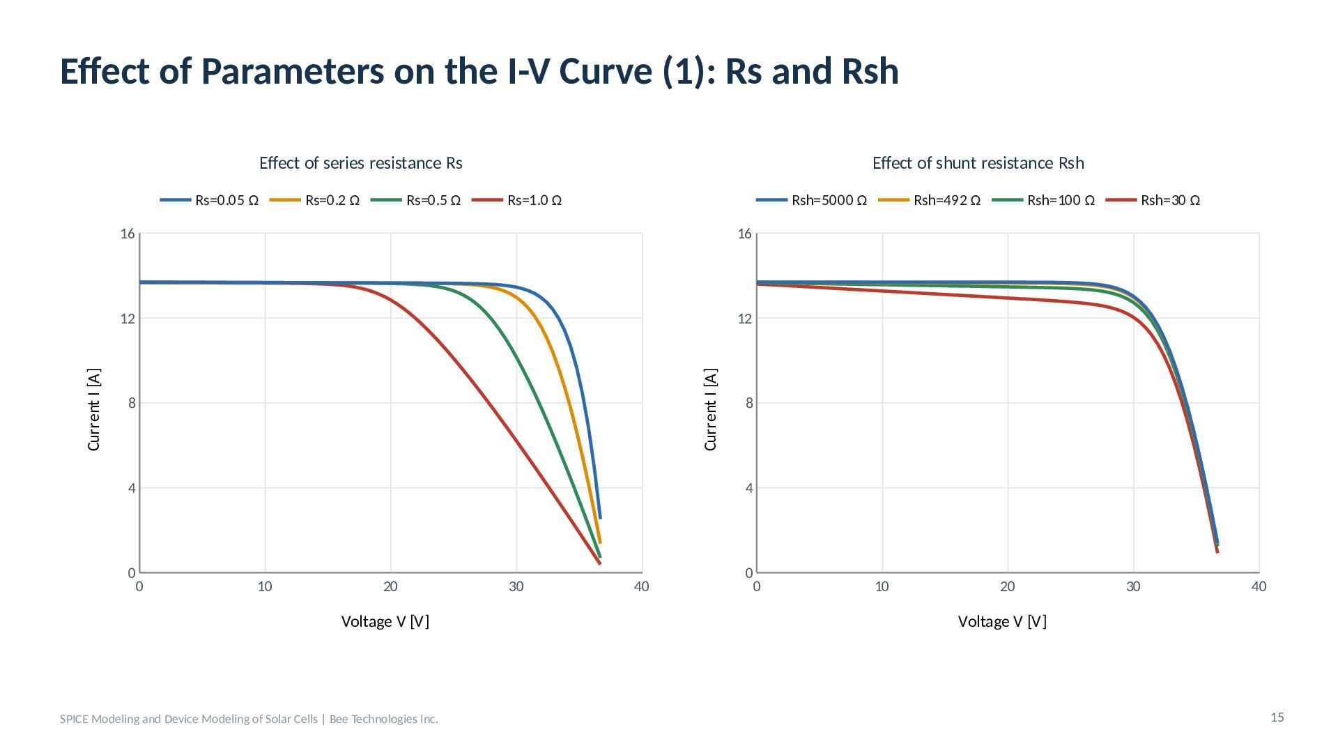
15. Effect of Parameters on the I-V Curve (1): Rs and Rsh Effect of series resistance Rs Rs=0.2 Ω Rs=0.5 Ω Rs=1.0 Ω Rsh=5000 Ω 16 16 12 12 Current I [A] Current I [A] Rs=0.05 Ω Effect of shunt resistance Rsh 8 4 0 0 Rsh=492 Ω Rsh=100 Ω Rsh=30 Ω 8 4 10 20 Voltage V [V] SPICE Modeling and Device Modeling of Solar Cells | Bee Technologies Inc. 30 40 0 0 10 20 30 40 Voltage V [V] 15
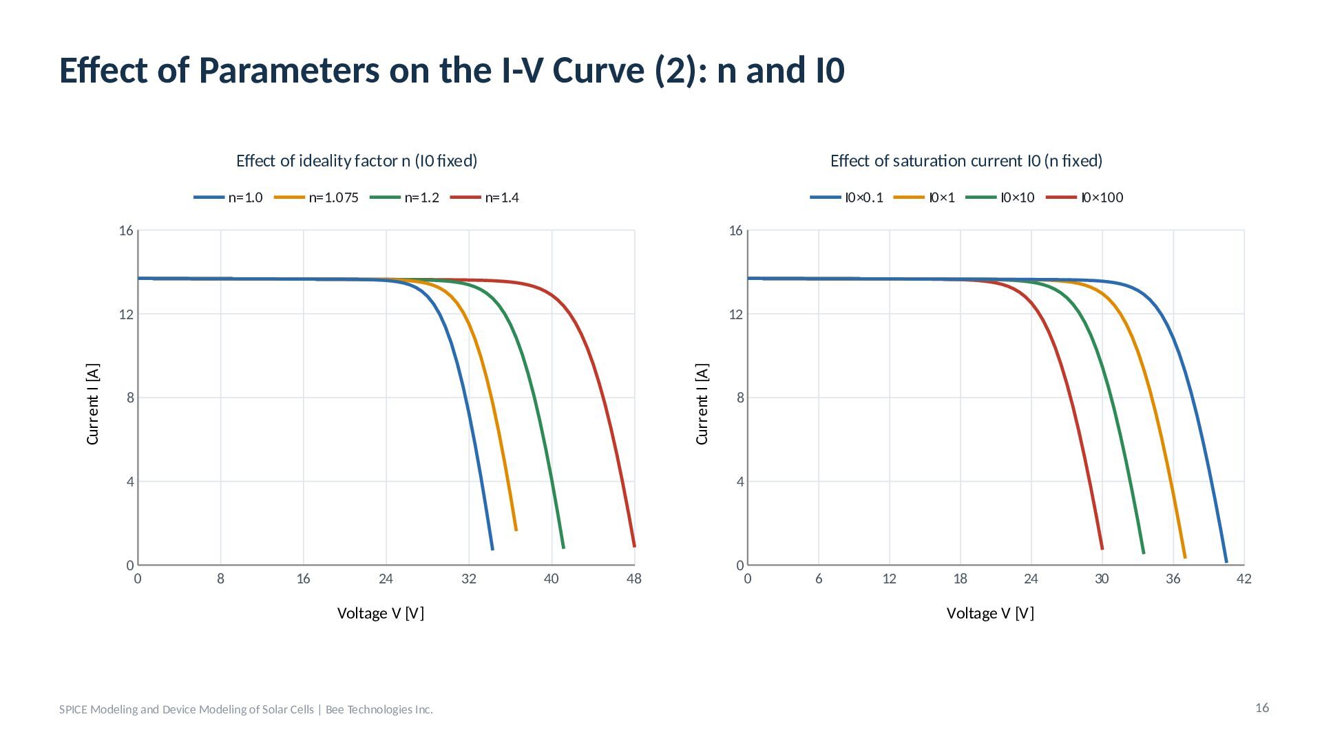
16. Effect of Parameters on the I-V Curve (2): n and I0 Effect of ideality factor n (I0 fixed) n=1.075 n=1.2 n=1.4 I0×0.1 16 16 12 12 Current I [A] Current I [A] n=1.0 Effect of saturation current I0 (n fixed) 8 4 0 0 I0×1 I0×10 I0×100 8 4 8 16 24 Voltage V [V] SPICE Modeling and Device Modeling of Solar Cells | Bee Technologies Inc. 32 40 48 0 0 6 12 18 24 30 36 42 Voltage V [V] 16
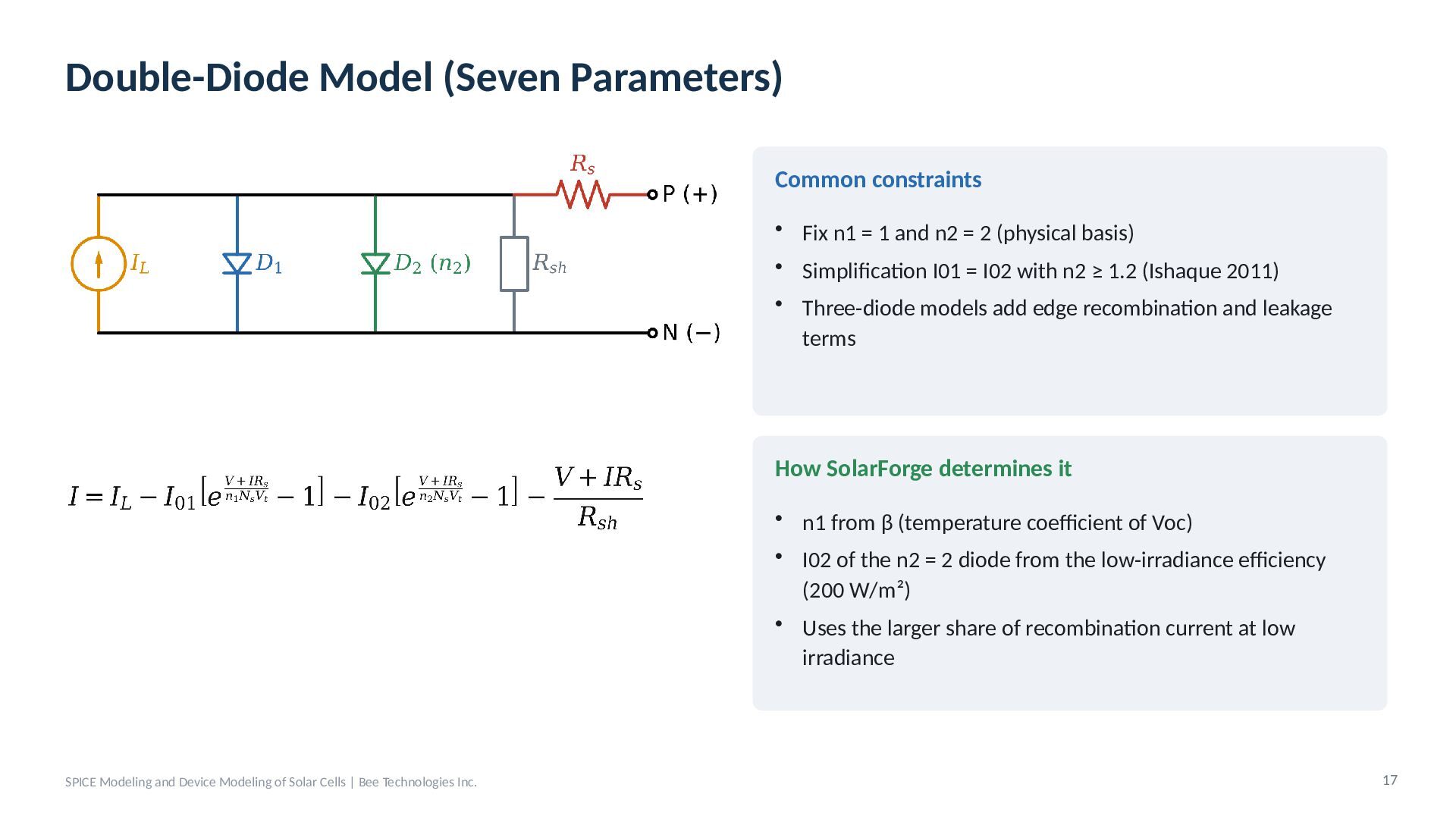
17. Double-Diode Model (Seven Parameters) Common constraints • Fix n1 = 1 and n2 = 2 (physical basis) • Simplification I01 = I02 with n2 ≥ 1.2 (Ishaque 2011) • Three-diode models add edge recombination and leakage terms How SolarForge determines it • n1 from β (temperature coefficient of Voc) • I02 of the n2 = 2 diode from the low-irradiance efficiency (200 W/m²) • Uses the larger share of recombination current at low irradiance SPICE Modeling and Device Modeling of Solar Cells | Bee Technologies Inc. 17
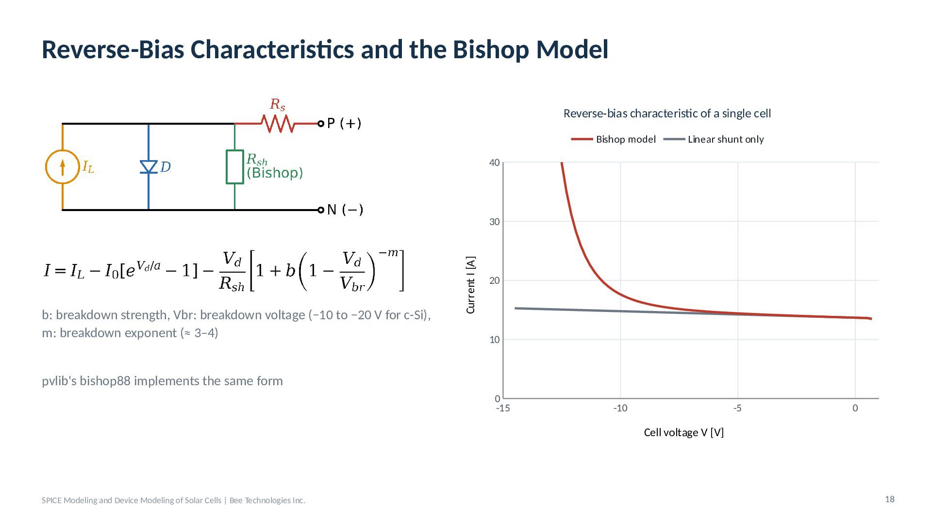
18. Reverse-Bias Characteristics and the Bishop Model Reverse-bias characteristic of a single cell Bishop model Linear shunt only 40 b: breakdown strength, Vbr: breakdown voltage (−10 to −20 V for c-Si), m: breakdown exponent (≈ 3–4) Current I [A] 30 20 10 pvlib's bishop88 implements the same form 0 -15 -10 -5 0 Cell voltage V [V] SPICE Modeling and Device Modeling of Solar Cells | Bee Technologies Inc. 18
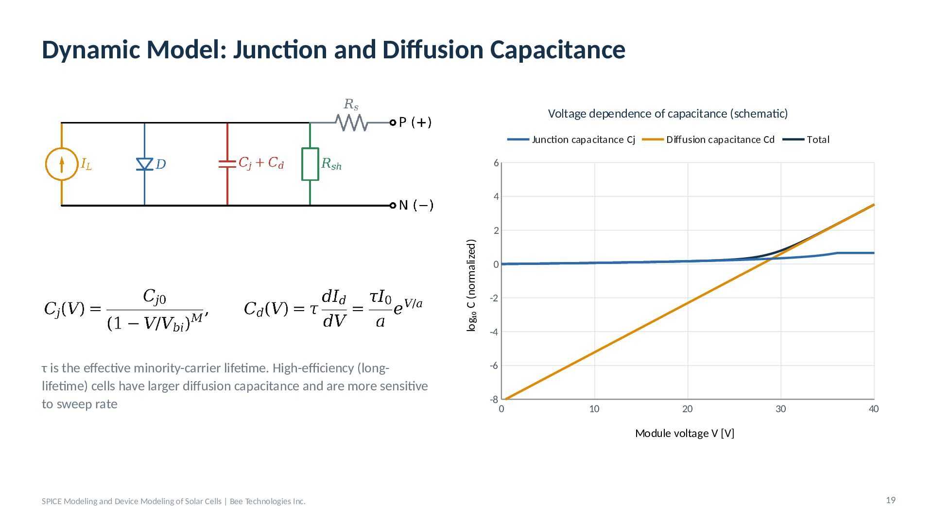
19. Dynamic Model: Junction and Diffusion Capacitance Voltage dependence of capacitance (schematic) Junction capacitance Cj Diffusion capacitance Cd Total 6 4 log₁₀ C (normalized) 2 τ is the effective minority-carrier lifetime. High-efficiency (longlifetime) cells have larger diffusion capacitance and are more sensitive to sweep rate 0 -2 -4 -6 -8 0 10 20 30 40 Module voltage V [V] SPICE Modeling and Device Modeling of Solar Cells | Bee Technologies Inc. 19
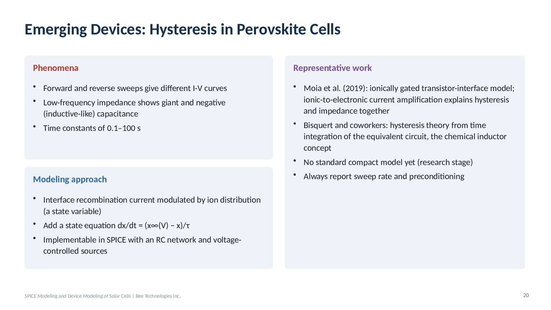
20. Emerging Devices: Hysteresis in Perovskite Cells Phenomena Representative work • Forward and reverse sweeps give different I-V curves • Low-frequency impedance shows giant and negative (inductive-like) capacitance • Time constants of 0.1–100 s • Moia et al. (2019): ionically gated transistor-interface model; ionic-to-electronic current amplification explains hysteresis and impedance together • Bisquert and coworkers: hysteresis theory from time integration of the equivalent circuit, the chemical inductor concept • No standard compact model yet (research stage) Modeling approach • Always report sweep rate and preconditioning • Interface recombination current modulated by ion distribution (a state variable) • Add a state equation dx/dt = (x∞(V) − x)/τ • Implementable in SPICE with an RC network and voltagecontrolled sources SPICE Modeling and Device Modeling of Solar Cells | Bee Technologies Inc. 20
21. 04 Solving the Implicit Equation Explicit Lambert W solution and robust numerical methods 21
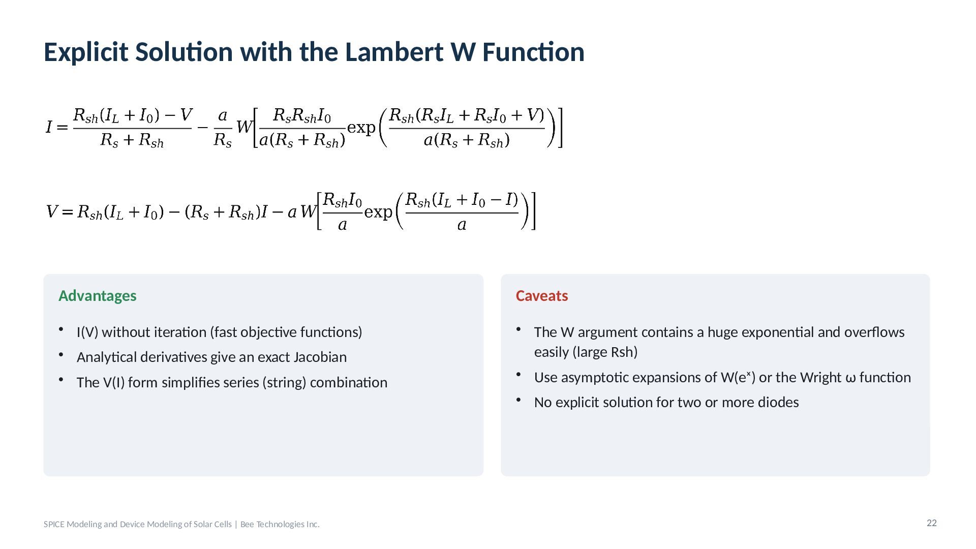
22. Explicit Solution with the Lambert W Function Advantages Caveats • I(V) without iteration (fast objective functions) • Analytical derivatives give an exact Jacobian • The W argument contains a huge exponential and overflows easily (large Rsh) • Use asymptotic expansions of W(eˣ) or the Wright ω function • The V(I) form simplifies series (string) combination SPICE Modeling and Device Modeling of Solar Cells | Bee Technologies Inc. • No explicit solution for two or more diodes 22
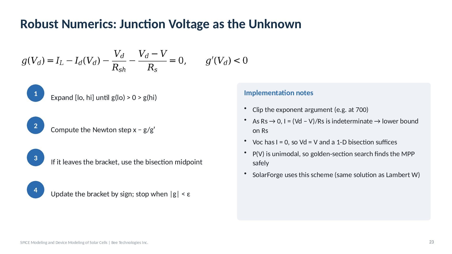
23. Robust Numerics: Junction Voltage as the Unknown 1 2 3 4 Expand [lo, hi] until g(lo) > 0 > g(hi) Compute the Newton step x − g/g′ If it leaves the bracket, use the bisection midpoint Implementation notes • Clip the exponent argument (e.g. at 700) • As Rs → 0, I = (Vd − V)/Rs is indeterminate → lower bound on Rs • Voc has I = 0, so Vd = V and a 1-D bisection suffices • P(V) is unimodal, so golden-section search finds the MPP safely • SolarForge uses this scheme (same solution as Lambert W) Update the bracket by sign; stop when |g| < ε SPICE Modeling and Device Modeling of Solar Cells | Bee Technologies Inc. 23
24. 05 Parameter Extraction Extraction from datasheets and fitting of measured I-V curves 24
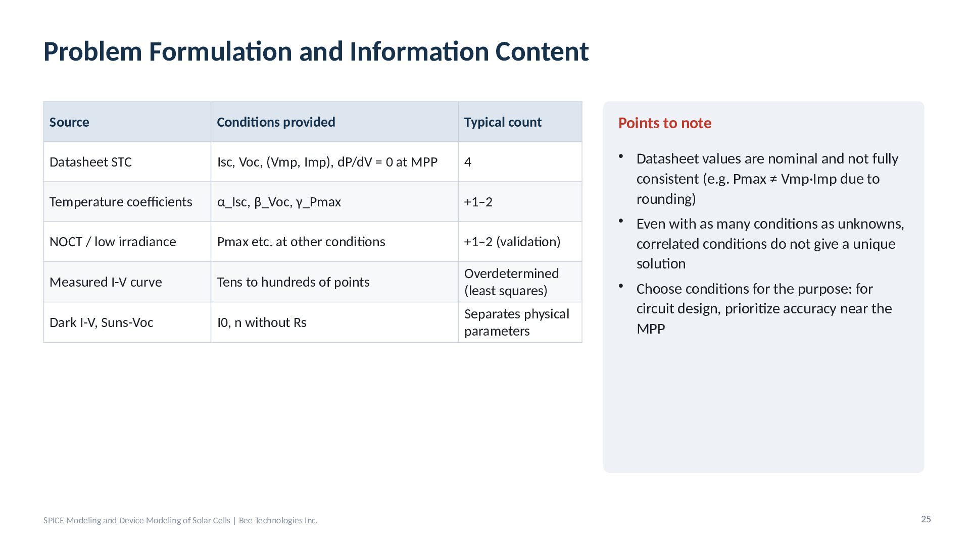
25. Problem Formulation and Information Content Source Conditions provided Typical count Points to note Datasheet STC Isc, Voc, (Vmp, Imp), dP/dV = 0 at MPP 4 Temperature coefficients α_Isc, β_Voc, γ_Pmax +1–2 NOCT / low irradiance Pmax etc. at other conditions +1–2 (validation) Measured I-V curve Tens to hundreds of points Overdetermined (least squares) Dark I-V, Suns-Voc I0, n without Rs Separates physical parameters • Datasheet values are nominal and not fully consistent (e.g. Pmax ≠ Vmp·Imp due to rounding) • Even with as many conditions as unknowns, correlated conditions do not give a unique solution • Choose conditions for the purpose: for circuit design, prioritize accuracy near the MPP SPICE Modeling and Device Modeling of Solar Cells | Bee Technologies Inc. 25
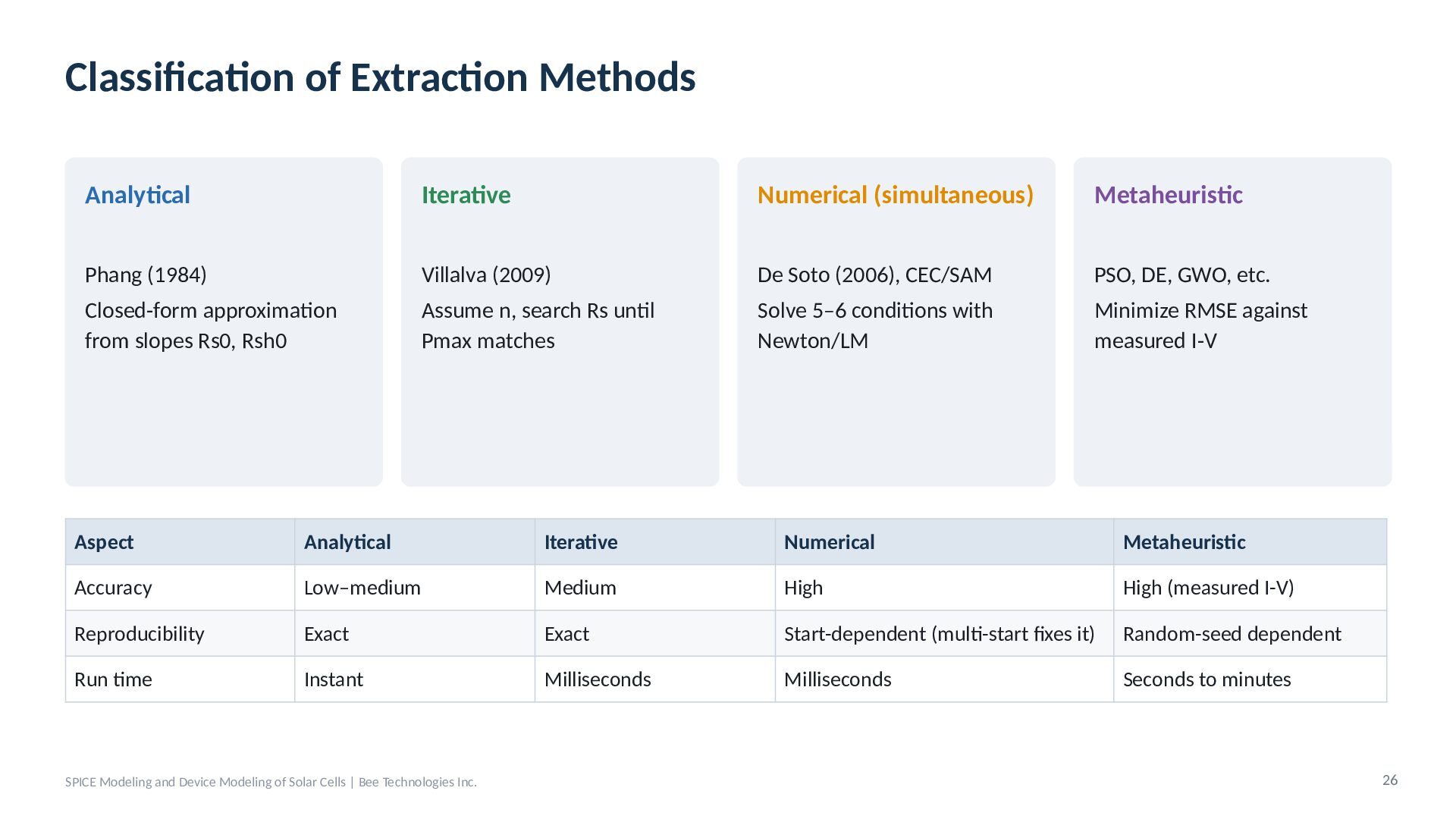
26. Classification of Extraction Methods Analytical Iterative Numerical (simultaneous) Metaheuristic Phang (1984) Villalva (2009) De Soto (2006), CEC/SAM PSO, DE, GWO, etc. Closed-form approximation from slopes Rs0, Rsh0 Assume n, search Rs until Pmax matches Solve 5–6 conditions with Newton/LM Minimize RMSE against measured I-V Aspect Analytical Iterative Numerical Metaheuristic Accuracy Low–medium Medium High High (measured I-V) Reproducibility Exact Exact Start-dependent (multi-start fixes it) Random-seed dependent Run time Instant Milliseconds Milliseconds Seconds to minutes SPICE Modeling and Device Modeling of Solar Cells | Bee Technologies Inc. 26
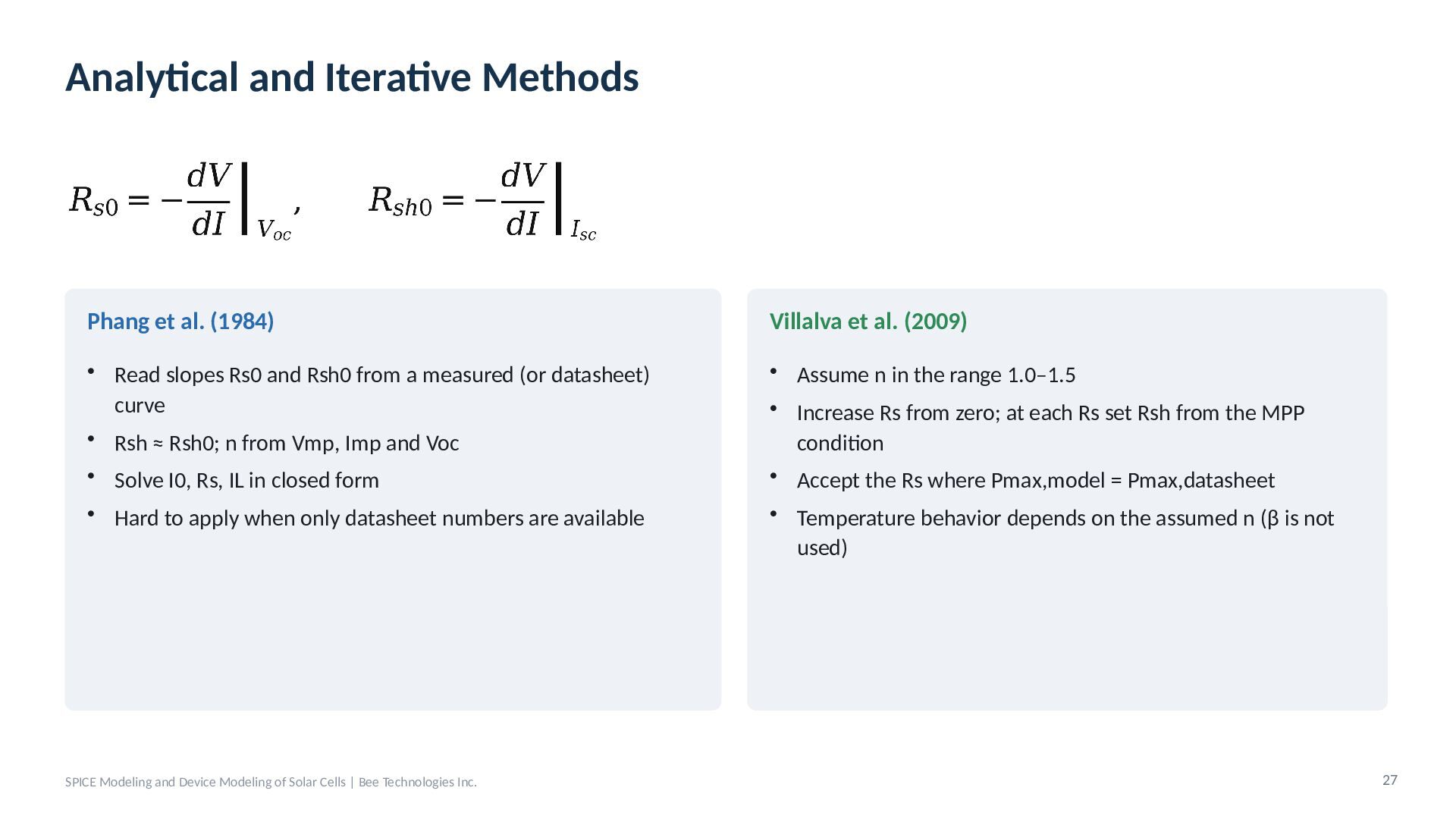
27. Analytical and Iterative Methods Phang et al. (1984) Villalva et al. (2009) • Read slopes Rs0 and Rsh0 from a measured (or datasheet) curve • Rsh ≈ Rsh0; n from Vmp, Imp and Voc • Assume n in the range 1.0–1.5 • Increase Rs from zero; at each Rs set Rsh from the MPP condition • Accept the Rs where Pmax,model = Pmax,datasheet • Solve I0, Rs, IL in closed form • Hard to apply when only datasheet numbers are available SPICE Modeling and Device Modeling of Solar Cells | Bee Technologies Inc. • Temperature behavior depends on the assumed n (β is not used) 27
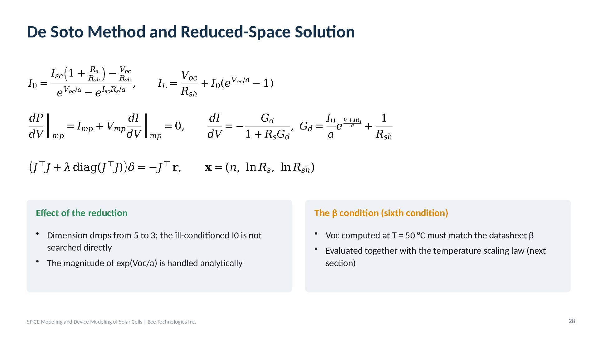
28. De Soto Method and Reduced-Space Solution Effect of the reduction The β condition (sixth condition) • Dimension drops from 5 to 3; the ill-conditioned I0 is not searched directly • The magnitude of exp(Voc/a) is handled analytically • Voc computed at T = 50 °C must match the datasheet β • Evaluated together with the temperature scaling law (next section) SPICE Modeling and Device Modeling of Solar Cells | Bee Technologies Inc. 28
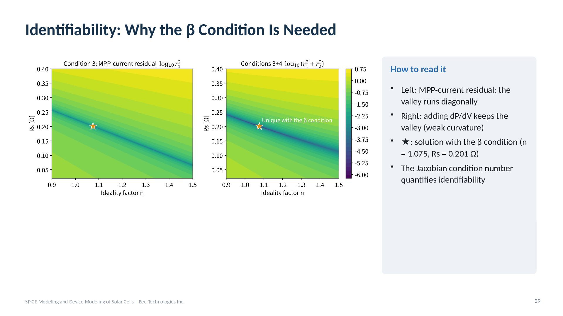
29. Identifiability: Why the β Condition Is Needed How to read it • Left: MPP-current residual; the valley runs diagonally • Right: adding dP/dV keeps the valley (weak curvature) • ★: solution with the β condition (n = 1.075, Rs = 0.201 Ω) • The Jacobian condition number quantifies identifiability SPICE Modeling and Device Modeling of Solar Cells | Bee Technologies Inc. 29
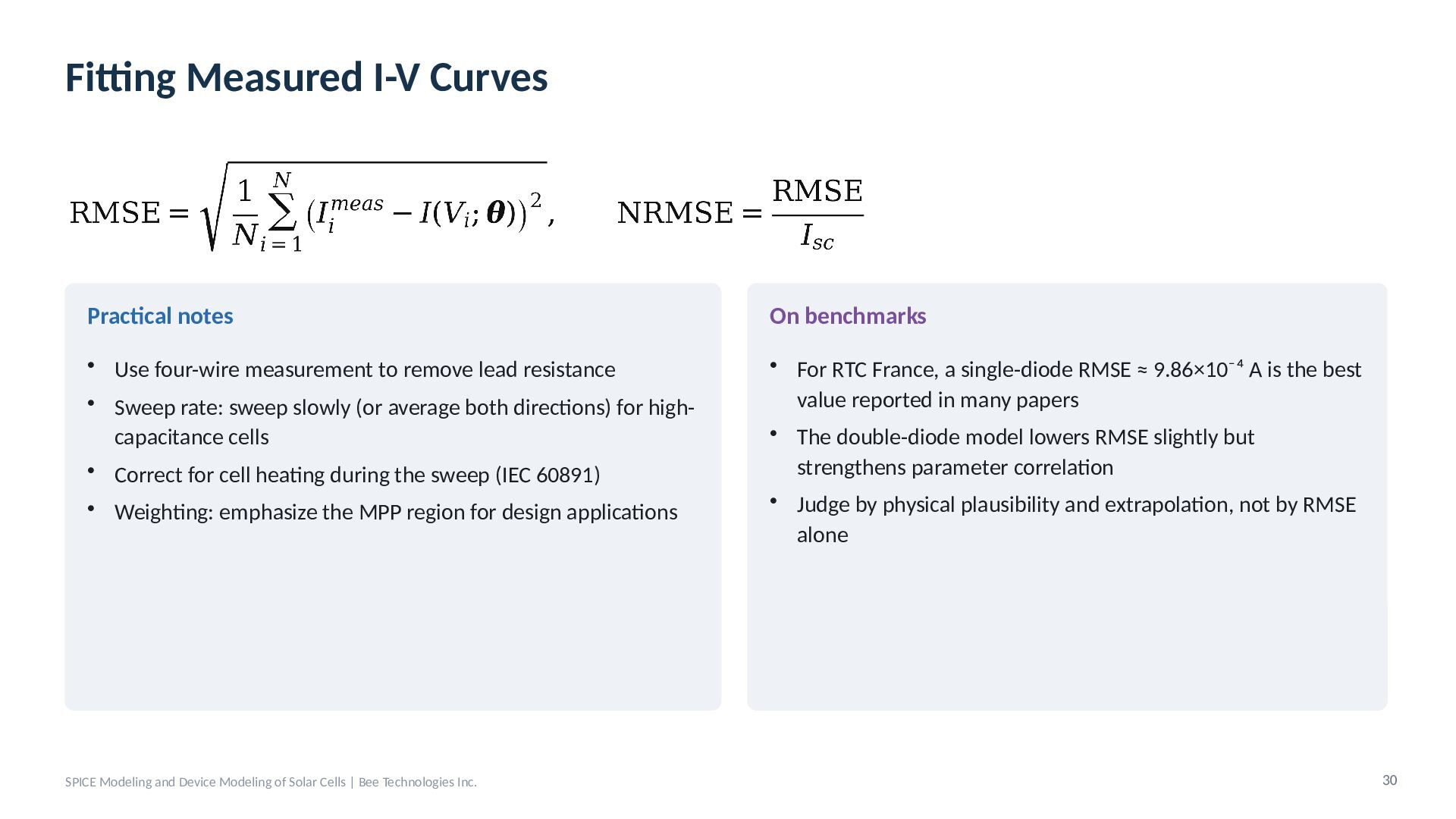
30. Fitting Measured I-V Curves Practical notes On benchmarks • Use four-wire measurement to remove lead resistance • Sweep rate: sweep slowly (or average both directions) for highcapacitance cells • Correct for cell heating during the sweep (IEC 60891) • For RTC France, a single-diode RMSE ≈ 9.86×10⁻⁴ A is the best value reported in many papers • The double-diode model lowers RMSE slightly but strengthens parameter correlation • Judge by physical plausibility and extrapolation, not by RMSE alone • Weighting: emphasize the MPP region for design applications SPICE Modeling and Device Modeling of Solar Cells | Bee Technologies Inc. 30
31. 06 Temperature, Irradiance, Spectrum Extrapolation laws and cell-temperature models 31
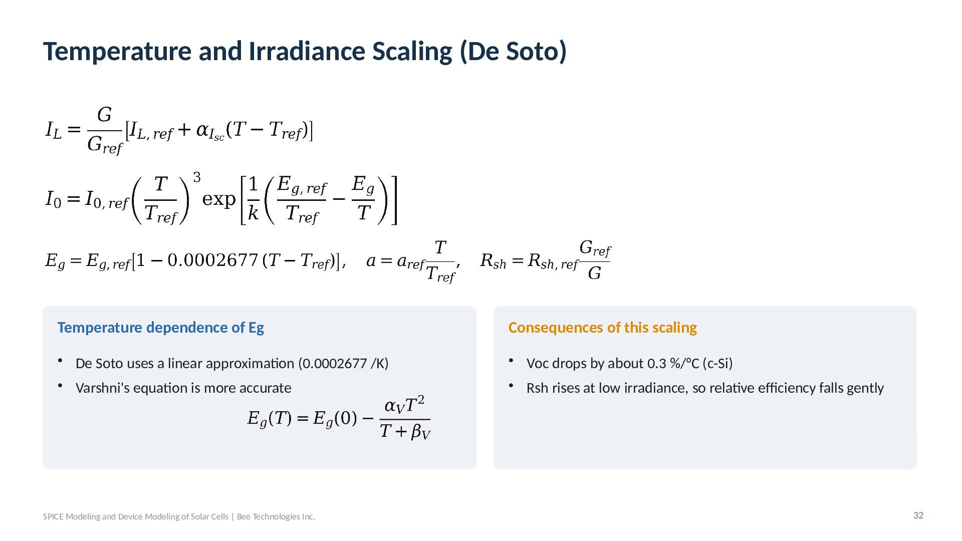
32. Temperature and Irradiance Scaling (De Soto) Temperature dependence of Eg Consequences of this scaling • De Soto uses a linear approximation (0.0002677 /K) • Varshni's equation is more accurate • Voc drops by about 0.3 %/°C (c-Si) • Rsh rises at low irradiance, so relative efficiency falls gently SPICE Modeling and Device Modeling of Solar Cells | Bee Technologies Inc. 32
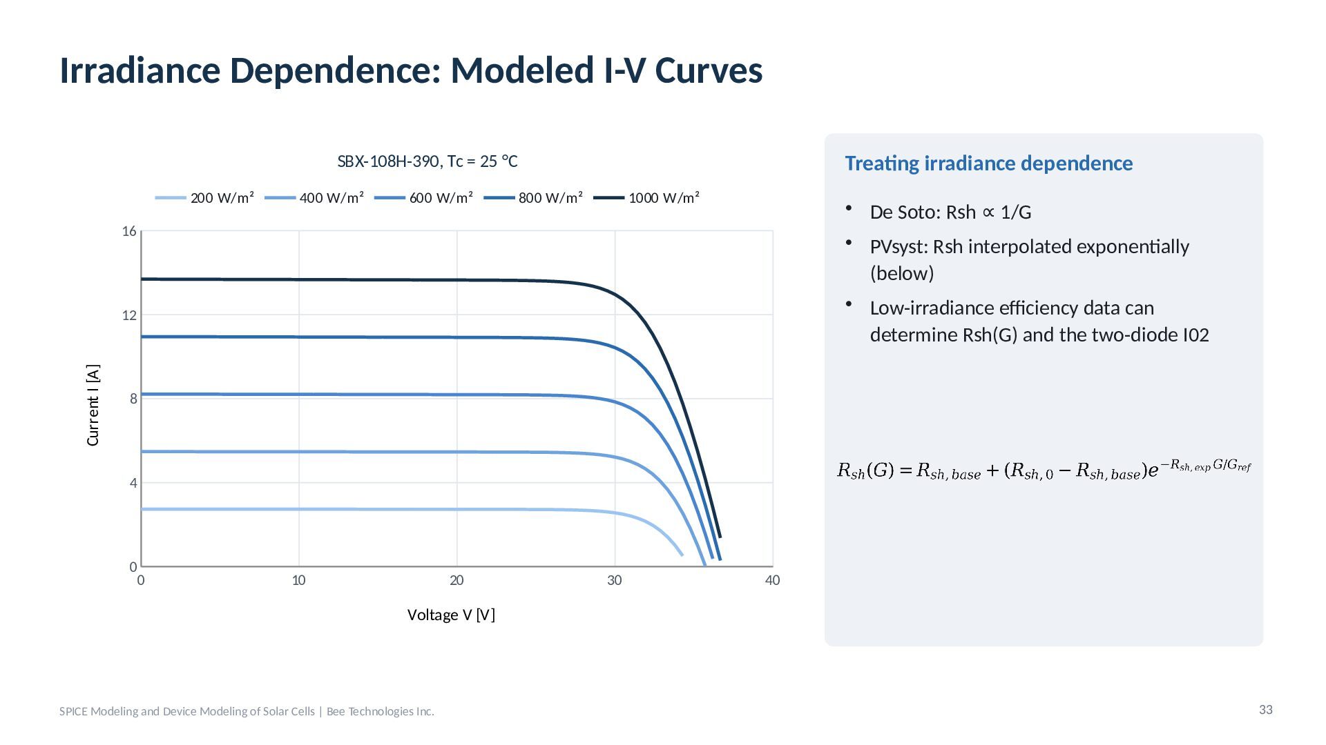
33. Irradiance Dependence: Modeled I-V Curves Treating irradiance dependence SBX-108H-390, Tc = 25 °C 200 W/m² 400 W/m² 600 W/m² 800 W/m² 1000 W/m² • De Soto: Rsh ∝ 1/G • PVsyst: Rsh interpolated exponentially (below) • Low-irradiance efficiency data can determine Rsh(G) and the two-diode I02 16 Current I [A] 12 8 4 0 0 10 20 30 40 Voltage V [V] SPICE Modeling and Device Modeling of Solar Cells | Bee Technologies Inc. 33
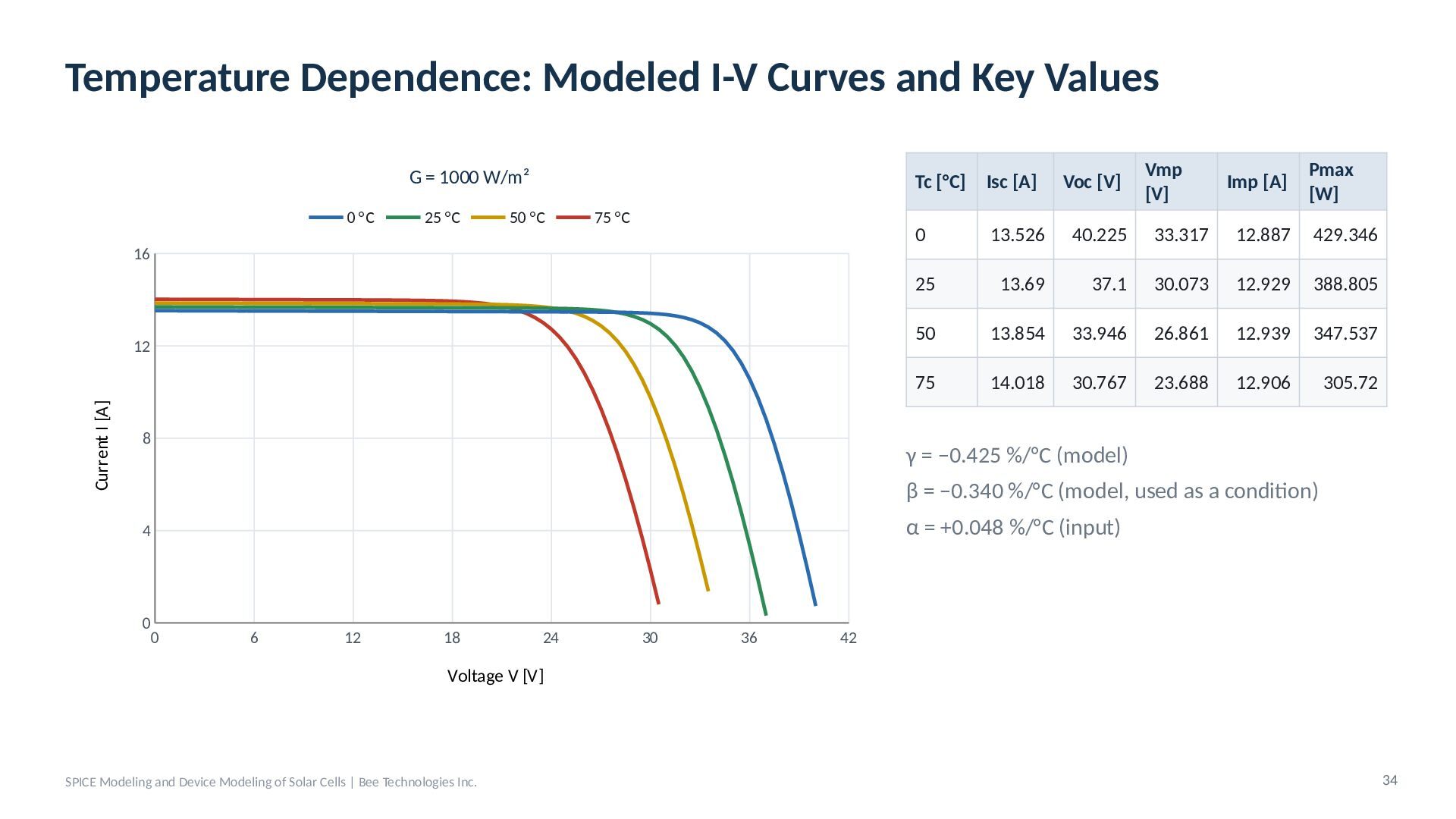
34. Temperature Dependence: Modeled I-V Curves and Key Values G = 1000 W/m² 0 °C 25 °C 50 °C 75 °C 16 Current I [A] 12 8 Tc [°C] Isc [A] Voc [V] Vmp [V] Imp [A] Pmax [W] 0 13.526 40.225 33.317 12.887 429.346 25 13.69 37.1 30.073 12.929 388.805 50 13.854 33.946 26.861 12.939 347.537 75 14.018 30.767 23.688 12.906 305.72 γ = −0.425 %/°C (model) β = −0.340 %/°C (model, used as a condition) α = +0.048 %/°C (input) 4 0 0 6 12 18 24 30 36 42 Voltage V [V] SPICE Modeling and Device Modeling of Solar Cells | Bee Technologies Inc. 34
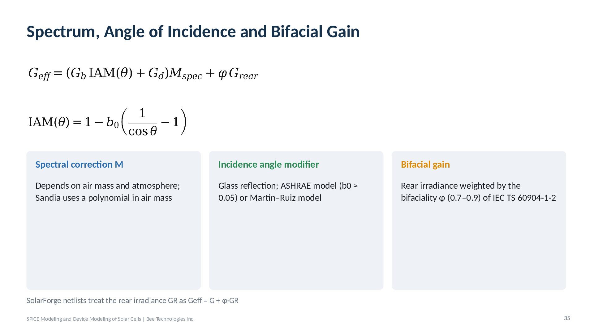
35. Spectrum, Angle of Incidence and Bifacial Gain Spectral correction M Incidence angle modifier Bifacial gain Depends on air mass and atmosphere; Sandia uses a polynomial in air mass Glass reflection; ASHRAE model (b0 ≈ 0.05) or Martin–Ruiz model Rear irradiance weighted by the bifaciality φ (0.7–0.9) of IEC TS 60904-1-2 SolarForge netlists treat the rear irradiance GR as Geff = G + φ·GR SPICE Modeling and Device Modeling of Solar Cells | Bee Technologies Inc. 35
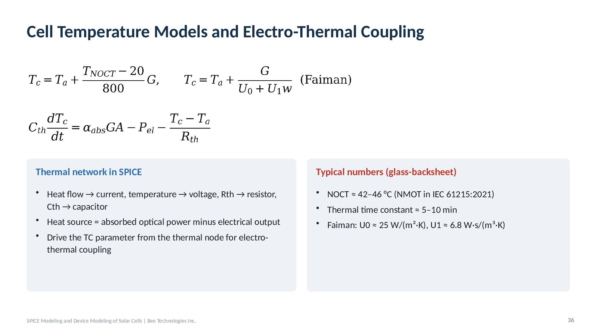
36. Cell Temperature Models and Electro-Thermal Coupling Thermal network in SPICE Typical numbers (glass-backsheet) • Heat flow → current, temperature → voltage, Rth → resistor, Cth → capacitor • Heat source = absorbed optical power minus electrical output • NOCT ≈ 42–46 °C (NMOT in IEC 61215:2021) • Thermal time constant ≈ 5–10 min • Drive the TC parameter from the thermal node for electrothermal coupling SPICE Modeling and Device Modeling of Solar Cells | Bee Technologies Inc. • Faiman: U0 ≈ 25 W/(m²·K), U1 ≈ 6.8 W·s/(m³·K) 36
37. 07 Modules and Arrays Cell-to-module scaling, mismatch, bypass diodes 37
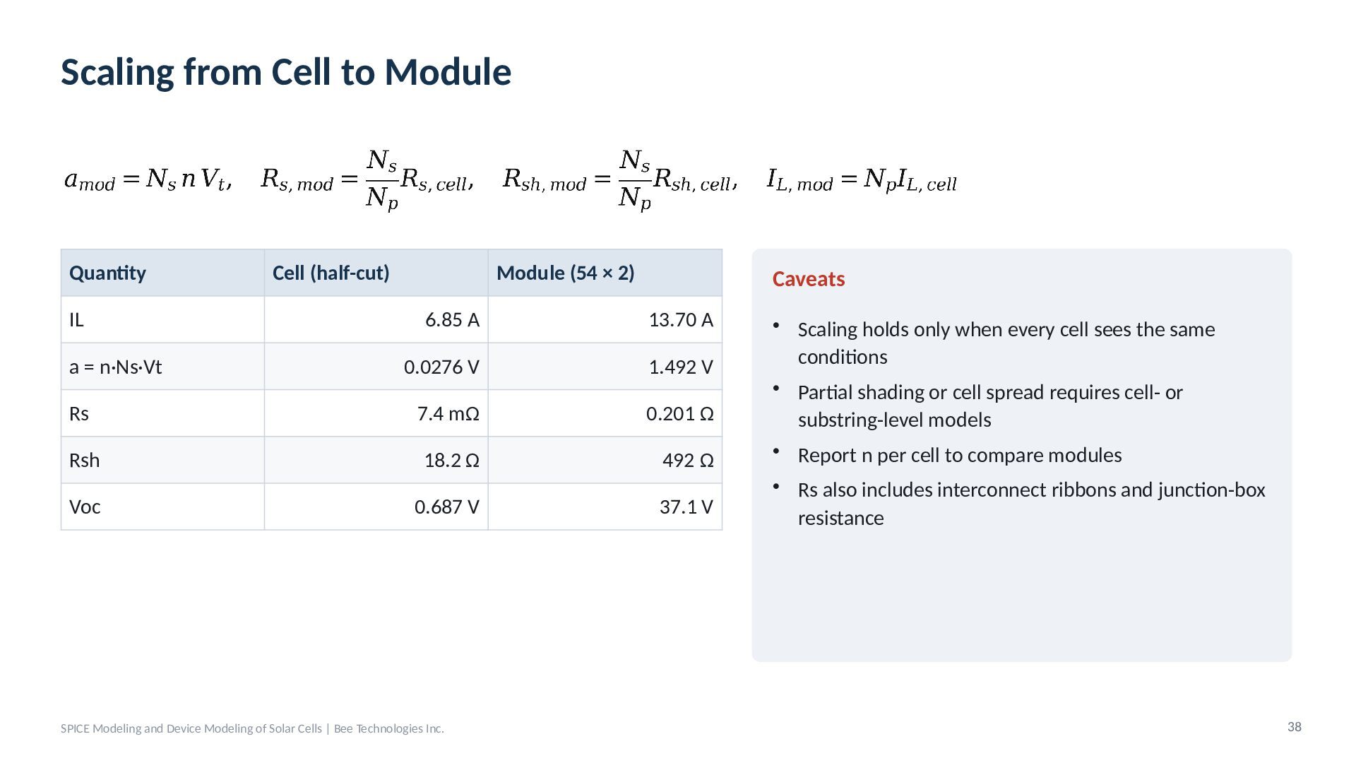
38. Scaling from Cell to Module Quantity IL Cell (half-cut) Module (54 × 2) Caveats 6.85 A 13.70 A a = n·Ns·Vt 0.0276 V 1.492 V Rs 7.4 mΩ 0.201 Ω Rsh 18.2 Ω 492 Ω Voc 0.687 V 37.1 V SPICE Modeling and Device Modeling of Solar Cells | Bee Technologies Inc. • Scaling holds only when every cell sees the same conditions • Partial shading or cell spread requires cell- or substring-level models • Report n per cell to compare modules • Rs also includes interconnect ribbons and junction-box resistance 38
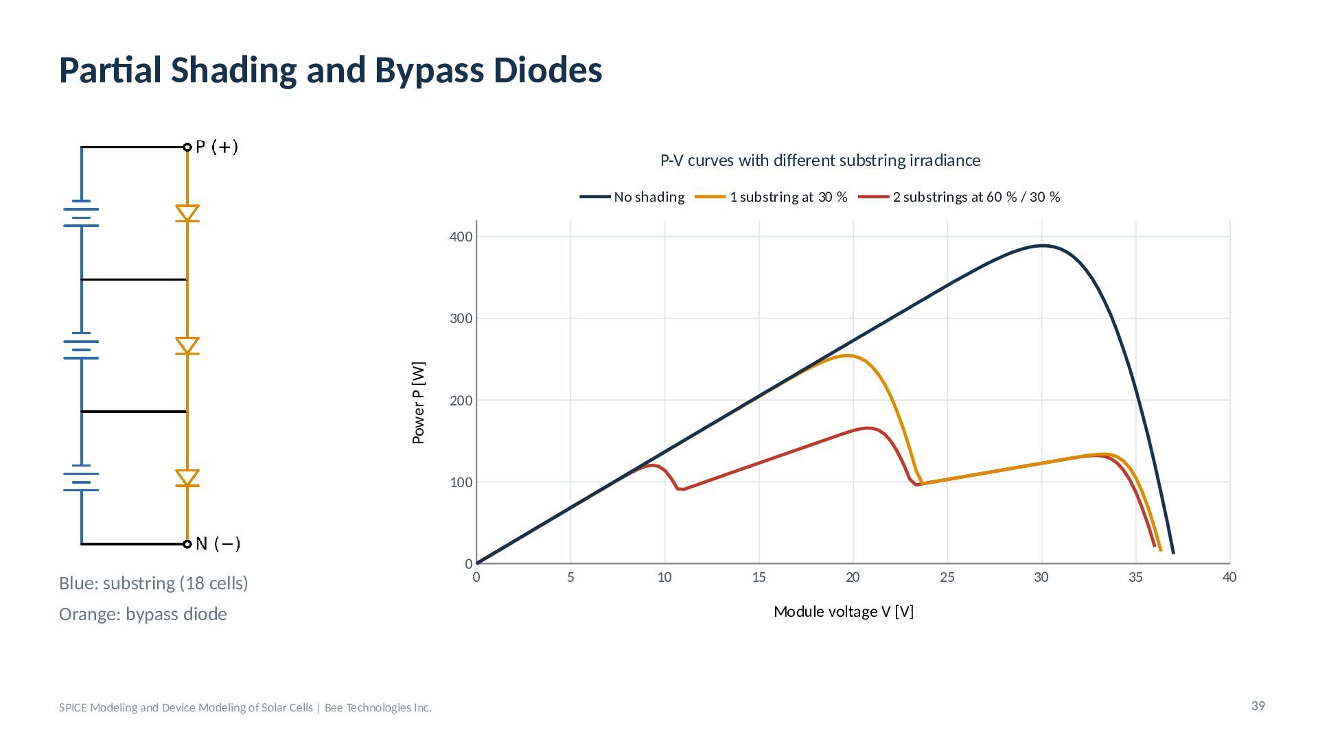
39. Partial Shading and Bypass Diodes P-V curves with different substring irradiance No shading 1 substring at 30 % 2 substrings at 60 % / 30 % 400 Power P [W] 300 200 100 Blue: substring (18 cells) Orange: bypass diode SPICE Modeling and Device Modeling of Solar Cells | Bee Technologies Inc. 0 0 5 10 15 20 25 30 35 40 Module voltage V [V] 39
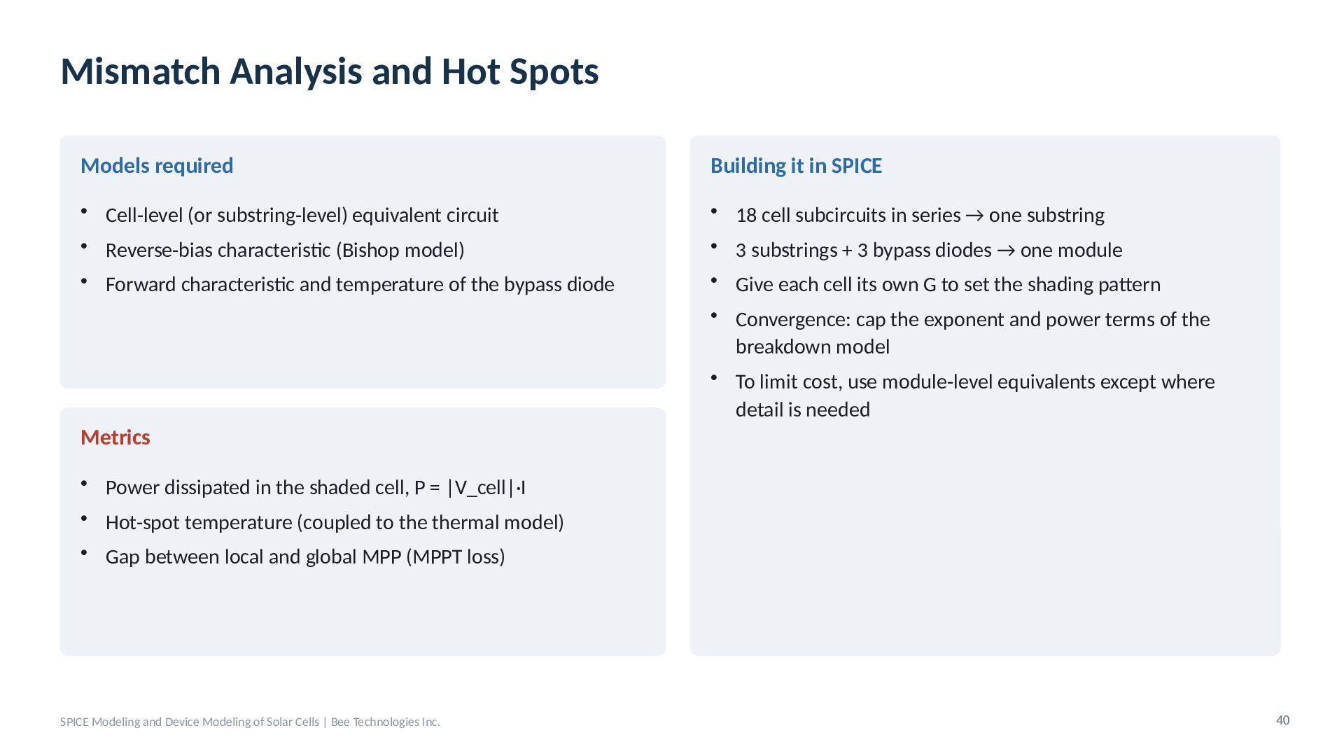
40. Mismatch Analysis and Hot Spots Models required Building it in SPICE • Cell-level (or substring-level) equivalent circuit • Reverse-bias characteristic (Bishop model) • 18 cell subcircuits in series → one substring • 3 substrings + 3 bypass diodes → one module • Forward characteristic and temperature of the bypass diode • Give each cell its own G to set the shading pattern • Convergence: cap the exponent and power terms of the breakdown model • To limit cost, use module-level equivalents except where detail is needed Metrics • Power dissipated in the shaded cell, P = |V_cell|·I • Hot-spot temperature (coupled to the thermal model) • Gap between local and global MPP (MPPT loss) SPICE Modeling and Device Modeling of Solar Cells | Bee Technologies Inc. 40
41. 08 SPICE Implementation Diode-model and behavioral approaches, convergence, applications 41
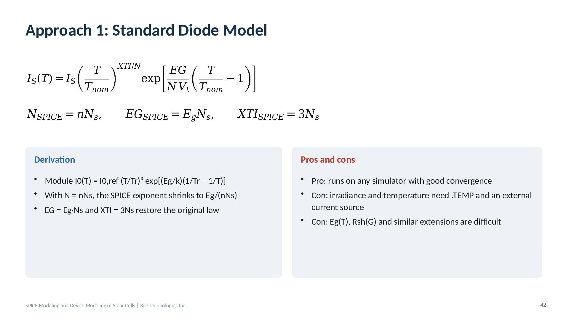
42. Approach 1: Standard Diode Model Derivation Pros and cons • Module I0(T) = I0,ref (T/Tr)³ exp[(Eg/k)(1/Tr − 1/T)] • With N = nNs, the SPICE exponent shrinks to Eg/(nNs) • Pro: runs on any simulator with good convergence • Con: irradiance and temperature need .TEMP and an external current source • Con: Eg(T), Rsh(G) and similar extensions are difficult • EG = Eg·Ns and XTI = 3Ns restore the original law SPICE Modeling and Device Modeling of Solar Cells | Bee Technologies Inc. 42
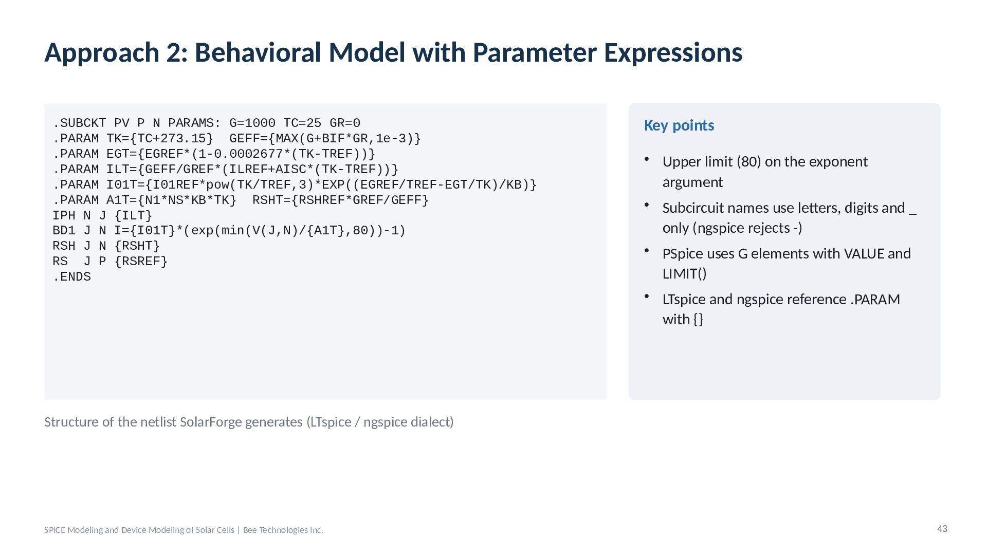
43. Approach 2: Behavioral Model with Parameter Expressions .SUBCKT PV P N PARAMS: G=1000 TC=25 GR=0 .PARAM TK={TC+273.15} GEFF={MAX(G+BIF*GR,1e-3)} .PARAM EGT={EGREF*(1-0.0002677*(TK-TREF))} .PARAM ILT={GEFF/GREF*(ILREF+AISC*(TK-TREF))} .PARAM I01T={I01REF*pow(TK/TREF,3)*EXP((EGREF/TREF-EGT/TK)/KB)} .PARAM A1T={N1*NS*KB*TK} RSHT={RSHREF*GREF/GEFF} IPH N J {ILT} BD1 J N I={I01T}*(exp(min(V(J,N)/{A1T},80))-1) RSH J N {RSHT} RS J P {RSREF} .ENDS Key points • Upper limit (80) on the exponent argument • Subcircuit names use letters, digits and _ only (ngspice rejects -) • PSpice uses G elements with VALUE and LIMIT() • LTspice and ngspice reference .PARAM with {} Structure of the netlist SolarForge generates (LTspice / ngspice dialect) SPICE Modeling and Device Modeling of Solar Cells | Bee Technologies Inc. 43
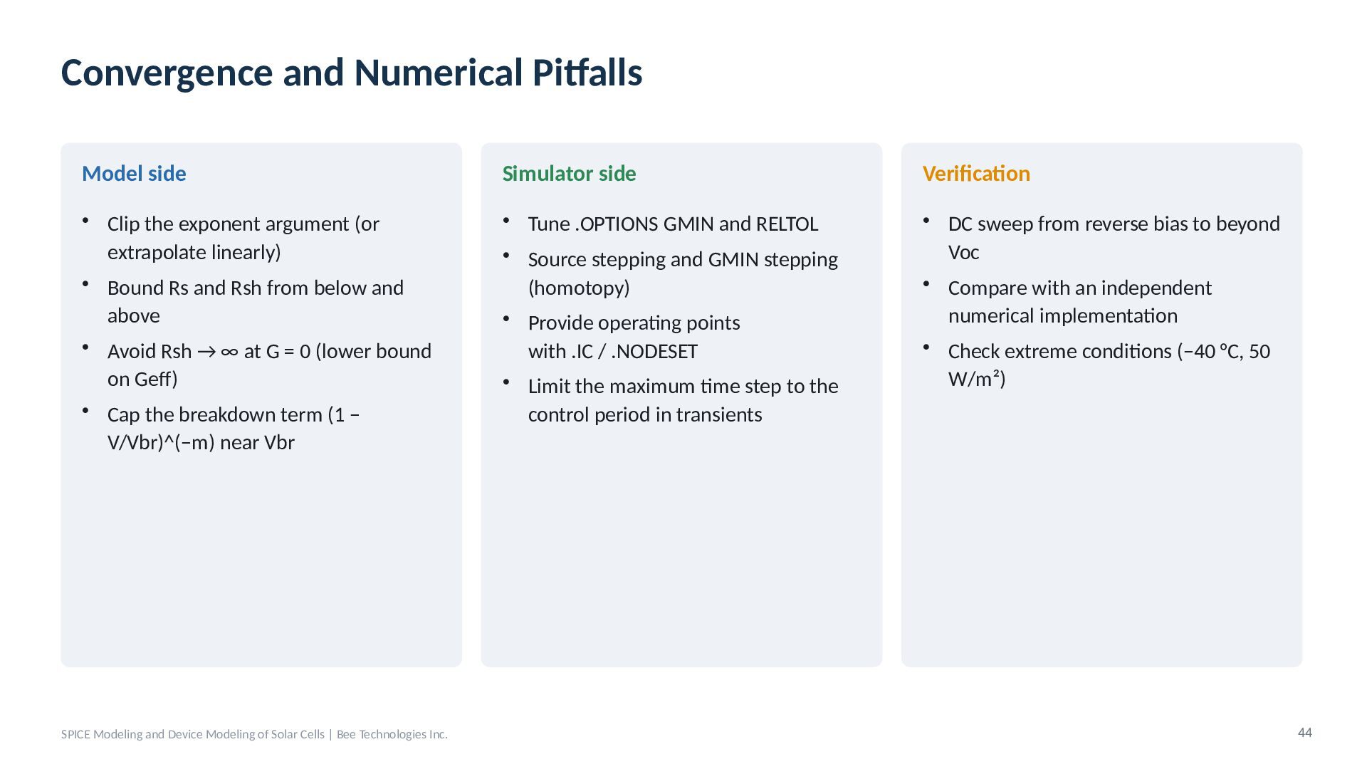
44. Convergence and Numerical Pitfalls Model side Simulator side Verification • Clip the exponent argument (or extrapolate linearly) • Bound Rs and Rsh from below and above • Avoid Rsh → ∞ at G = 0 (lower bound on Geff) • Cap the breakdown term (1 − V/Vbr)^(−m) near Vbr • Tune .OPTIONS GMIN and RELTOL • Source stepping and GMIN stepping (homotopy) • Provide operating points with .IC / .NODESET • Limit the maximum time step to the control period in transients • DC sweep from reverse bias to beyond Voc • Compare with an independent numerical implementation • Check extreme conditions (−40 °C, 50 W/m²) SPICE Modeling and Device Modeling of Solar Cells | Bee Technologies Inc. 44
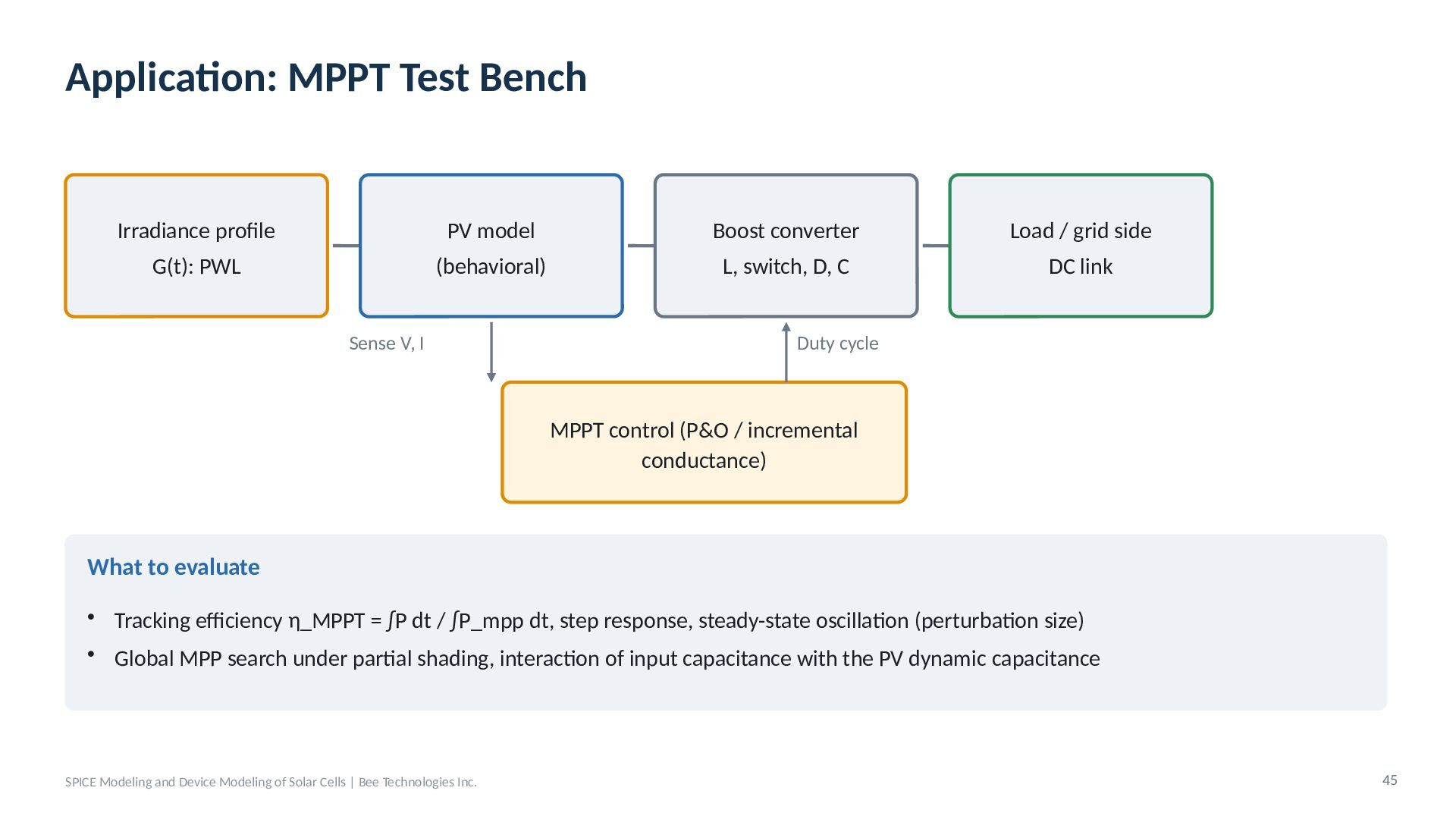
45. Application: MPPT Test Bench Irradiance profile PV model Boost converter Load / grid side G(t): PWL (behavioral) L, switch, D, C DC link Sense V, I Duty cycle MPPT control (P&O / incremental conductance) What to evaluate • Tracking efficiency η_MPPT = ∫P dt / ∫P_mpp dt, step response, steady-state oscillation (perturbation size) • Global MPP search under partial shading, interaction of input capacitance with the PV dynamic capacitance SPICE Modeling and Device Modeling of Solar Cells | Bee Technologies Inc. 45
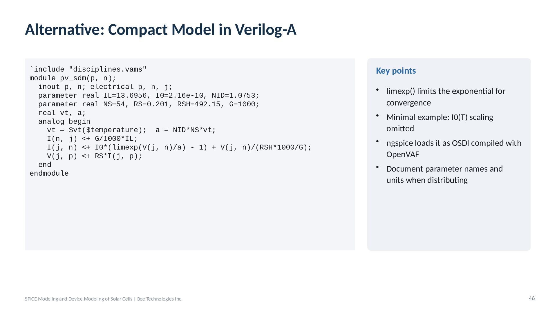
46. Alternative: Compact Model in Verilog-A `include "disciplines.vams" module pv_sdm(p, n); inout p, n; electrical p, n, j; parameter real IL=13.6956, I0=2.16e-10, NID=1.0753; parameter real NS=54, RS=0.201, RSH=492.15, G=1000; real vt, a; analog begin vt = $vt($temperature); a = NID*NS*vt; I(n, j) <+ G/1000*IL; I(j, n) <+ I0*(limexp(V(j, n)/a) - 1) + V(j, n)/(RSH*1000/G); V(j, p) <+ RS*I(j, p); end endmodule SPICE Modeling and Device Modeling of Solar Cells | Bee Technologies Inc. Key points • limexp() limits the exponential for convergence • Minimal example: I0(T) scaling omitted • ngspice loads it as OSDI compiled with OpenVAF • Document parameter names and units when distributing 46
47. 09 Validation and Quality Assurance Error metrics, cross-checks, the device modeling report 47
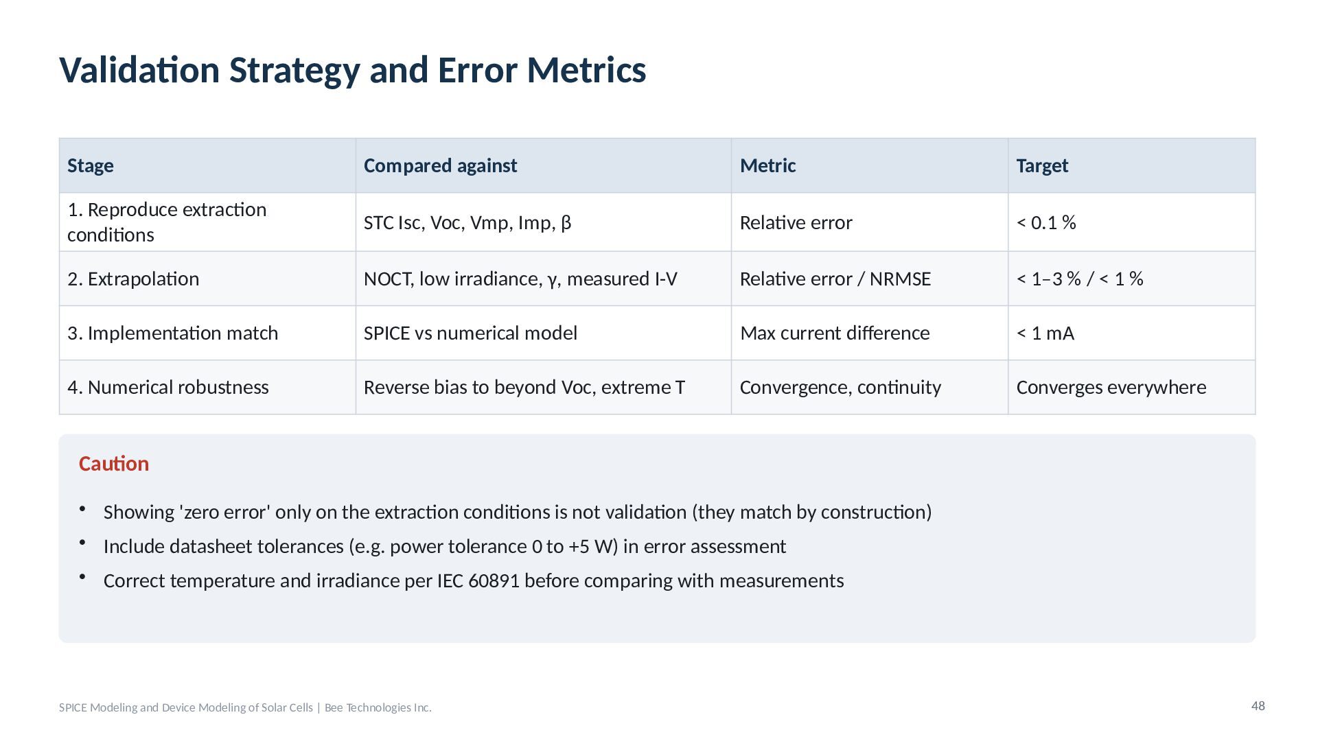
48. Validation Strategy and Error Metrics Stage Compared against Metric Target 1. Reproduce extraction conditions STC Isc, Voc, Vmp, Imp, β Relative error < 0.1 % 2. Extrapolation NOCT, low irradiance, γ, measured I-V Relative error / NRMSE < 1–3 % / < 1 % 3. Implementation match SPICE vs numerical model Max current difference < 1 mA 4. Numerical robustness Reverse bias to beyond Voc, extreme T Convergence, continuity Converges everywhere Caution • Showing 'zero error' only on the extraction conditions is not validation (they match by construction) • Include datasheet tolerances (e.g. power tolerance 0 to +5 W) in error assessment • Correct temperature and irradiance per IEC 60891 before comparing with measurements SPICE Modeling and Device Modeling of Solar Cells | Bee Technologies Inc. 48
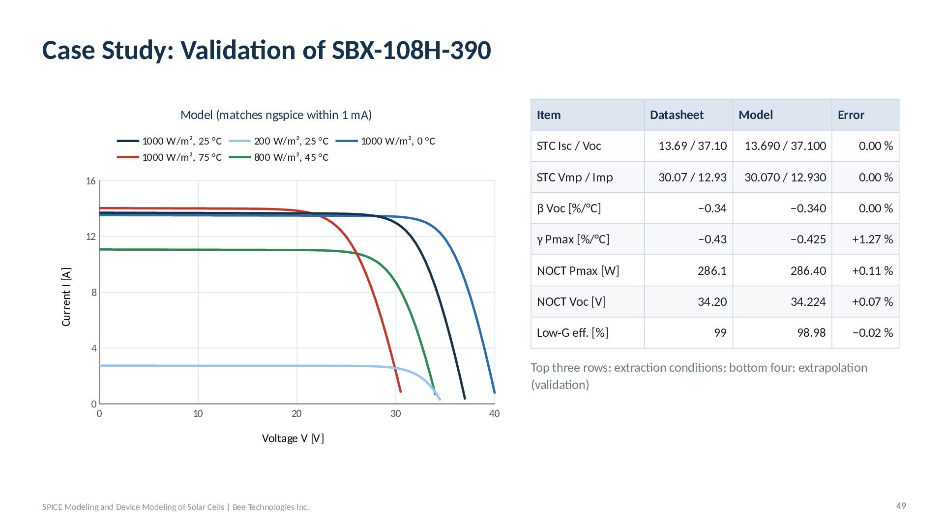
49. Case Study: Validation of SBX-108H-390 Model (matches ngspice within 1 mA) 1000 W/m², 25 °C 1000 W/m², 75 °C 200 W/m², 25 °C 800 W/m², 45 °C 1000 W/m², 0 °C 16 Current I [A] 12 8 Item Datasheet Model Error STC Isc / Voc 13.69 / 37.10 13.690 / 37.100 0.00 % STC Vmp / Imp 30.07 / 12.93 30.070 / 12.930 0.00 % β Voc [%/°C] −0.34 −0.340 0.00 % γ Pmax [%/°C] −0.43 −0.425 +1.27 % NOCT Pmax [W] 286.1 286.40 +0.11 % NOCT Voc [V] 34.20 34.224 +0.07 % Low-G eff. [%] 99 98.98 −0.02 % 4 Top three rows: extraction conditions; bottom four: extrapolation (validation) 0 0 10 20 30 40 Voltage V [V] SPICE Modeling and Device Modeling of Solar Cells | Bee Technologies Inc. 49
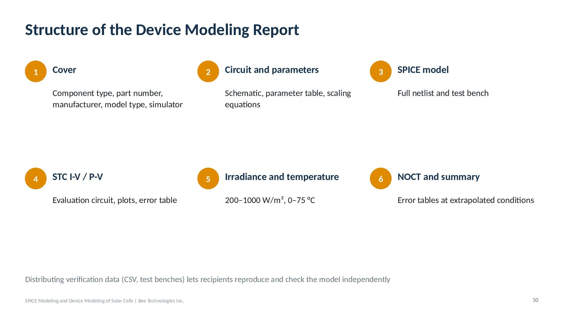
50. Structure of the Device Modeling Report 1 Cover 2 Component type, part number, manufacturer, model type, simulator 4 STC I-V / P-V Evaluation circuit, plots, error table Circuit and parameters 3 Schematic, parameter table, scaling equations 5 Irradiance and temperature SPICE model Full netlist and test bench 6 200–1000 W/m², 0–75 °C NOCT and summary Error tables at extrapolated conditions Distributing verification data (CSV, test benches) lets recipients reproduce and check the model independently SPICE Modeling and Device Modeling of Solar Cells | Bee Technologies Inc. 50
51. 10 Extensions to Emerging Devices High-efficiency Si, tandems, degradation, machine learning 51
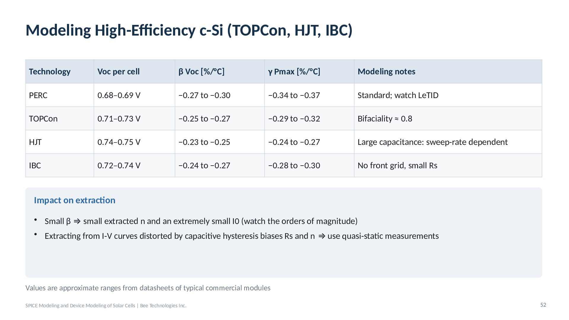
52. Modeling High-Efficiency c-Si (TOPCon, HJT, IBC) Technology Voc per cell β Voc [%/°C] γ Pmax [%/°C] Modeling notes PERC 0.68–0.69 V −0.27 to −0.30 −0.34 to −0.37 Standard; watch LeTID TOPCon 0.71–0.73 V −0.25 to −0.27 −0.29 to −0.32 Bifaciality ≈ 0.8 HJT 0.74–0.75 V −0.23 to −0.25 −0.24 to −0.27 Large capacitance: sweep-rate dependent IBC 0.72–0.74 V −0.24 to −0.27 −0.28 to −0.30 No front grid, small Rs Impact on extraction • Small β ⇒ small extracted n and an extremely small I0 (watch the orders of magnitude) • Extracting from I-V curves distorted by capacitive hysteresis biases Rs and n ⇒ use quasi-static measurements Values are approximate ranges from datasheets of typical commercial modules SPICE Modeling and Device Modeling of Solar Cells | Bee Technologies Inc. 52
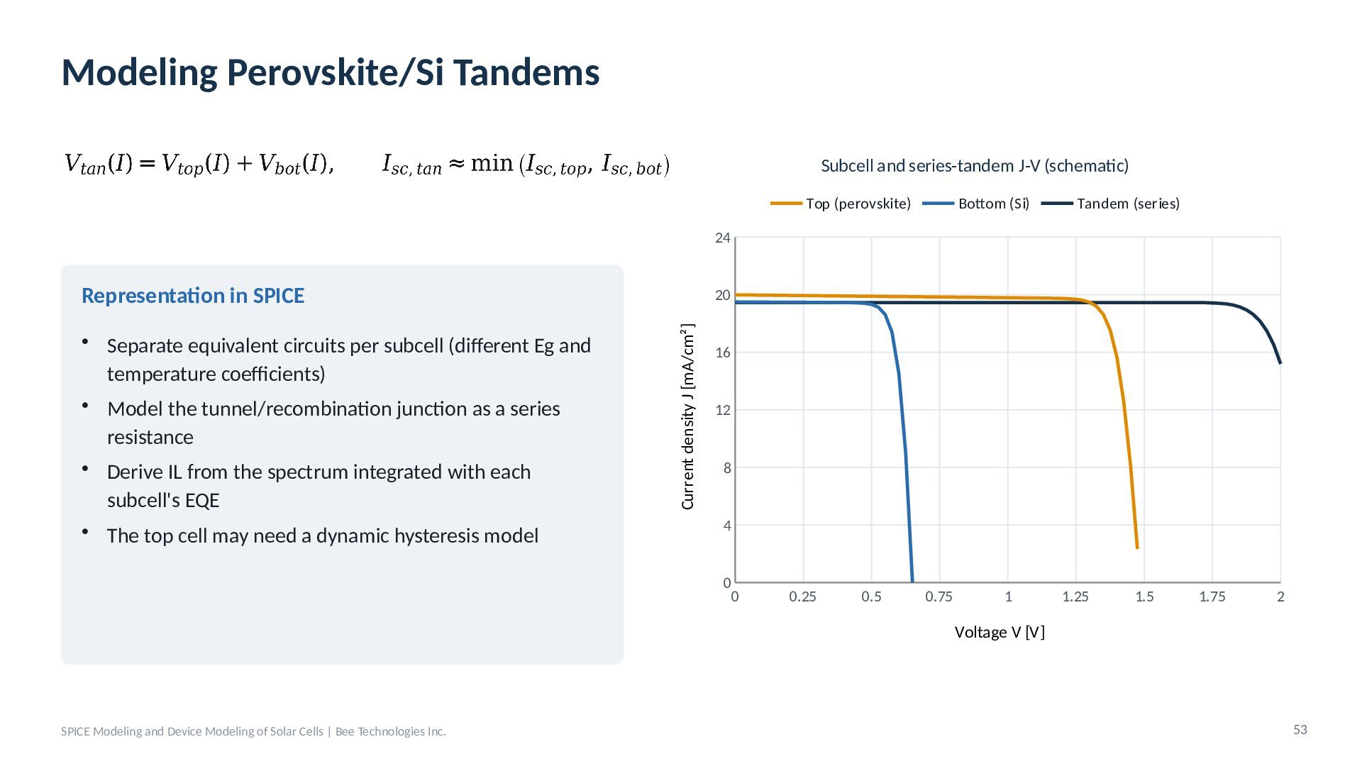
53. Modeling Perovskite/Si Tandems Subcell and series-tandem J-V (schematic) Top (perovskite) Bottom (Si) Tandem (series) 24 Representation in SPICE Current density J [mA/cm²] • Separate equivalent circuits per subcell (different Eg and temperature coefficients) • Model the tunnel/recombination junction as a series resistance • Derive IL from the spectrum integrated with each subcell's EQE • The top cell may need a dynamic hysteresis model 20 16 12 8 4 0 0 0.25 0.5 0.75 1 1.25 1.5 1.75 2 Voltage V [V] SPICE Modeling and Device Modeling of Solar Cells | Bee Technologies Inc. 53
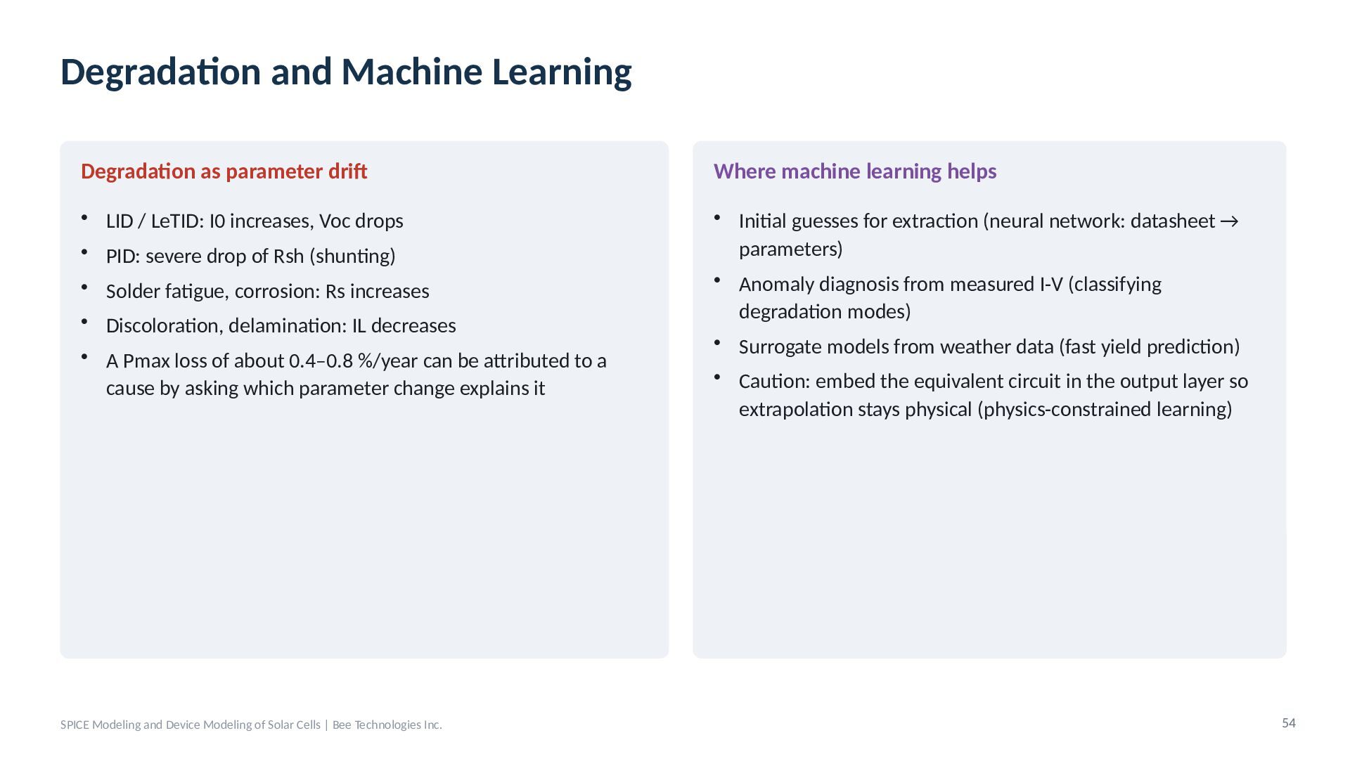
54. Degradation and Machine Learning Degradation as parameter drift Where machine learning helps • LID / LeTID: I0 increases, Voc drops • PID: severe drop of Rsh (shunting) • Initial guesses for extraction (neural network: datasheet → parameters) • Anomaly diagnosis from measured I-V (classifying degradation modes) • Surrogate models from weather data (fast yield prediction) • Solder fatigue, corrosion: Rs increases • Discoloration, delamination: IL decreases • A Pmax loss of about 0.4–0.8 %/year can be attributed to a cause by asking which parameter change explains it SPICE Modeling and Device Modeling of Solar Cells | Bee Technologies Inc. • Caution: embed the equivalent circuit in the output layer so extrapolation stays physical (physics-constrained learning) 54
55. 11 Summary and Exercises Key points, exercises, references 55
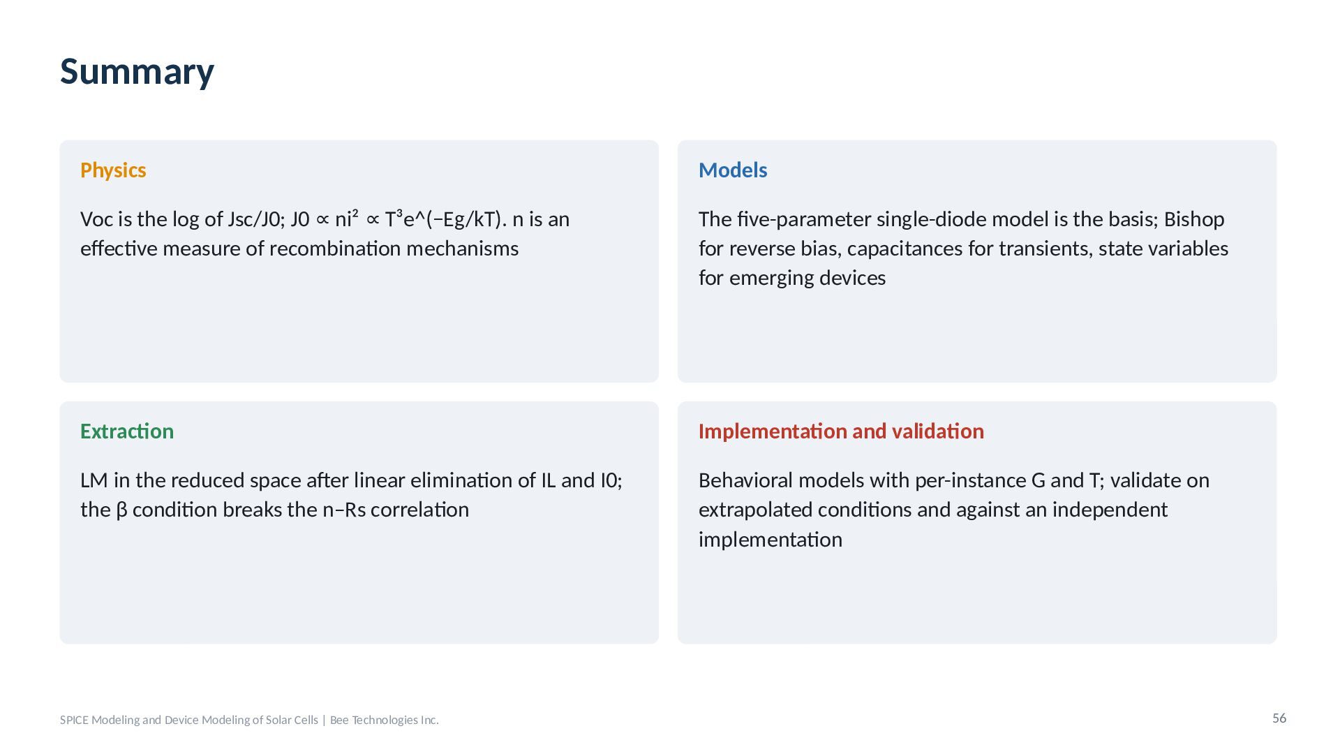
56. Summary Physics Models Voc is the log of Jsc/J0; J0 ∝ ni² ∝ T³e^(−Eg/kT). n is an effective measure of recombination mechanisms The five-parameter single-diode model is the basis; Bishop for reverse bias, capacitances for transients, state variables for emerging devices Extraction Implementation and validation LM in the reduced space after linear elimination of IL and I0; the β condition breaks the n–Rs correlation Behavioral models with per-instance G and T; validate on extrapolated conditions and against an independent implementation SPICE Modeling and Device Modeling of Solar Cells | Bee Technologies Inc. 56
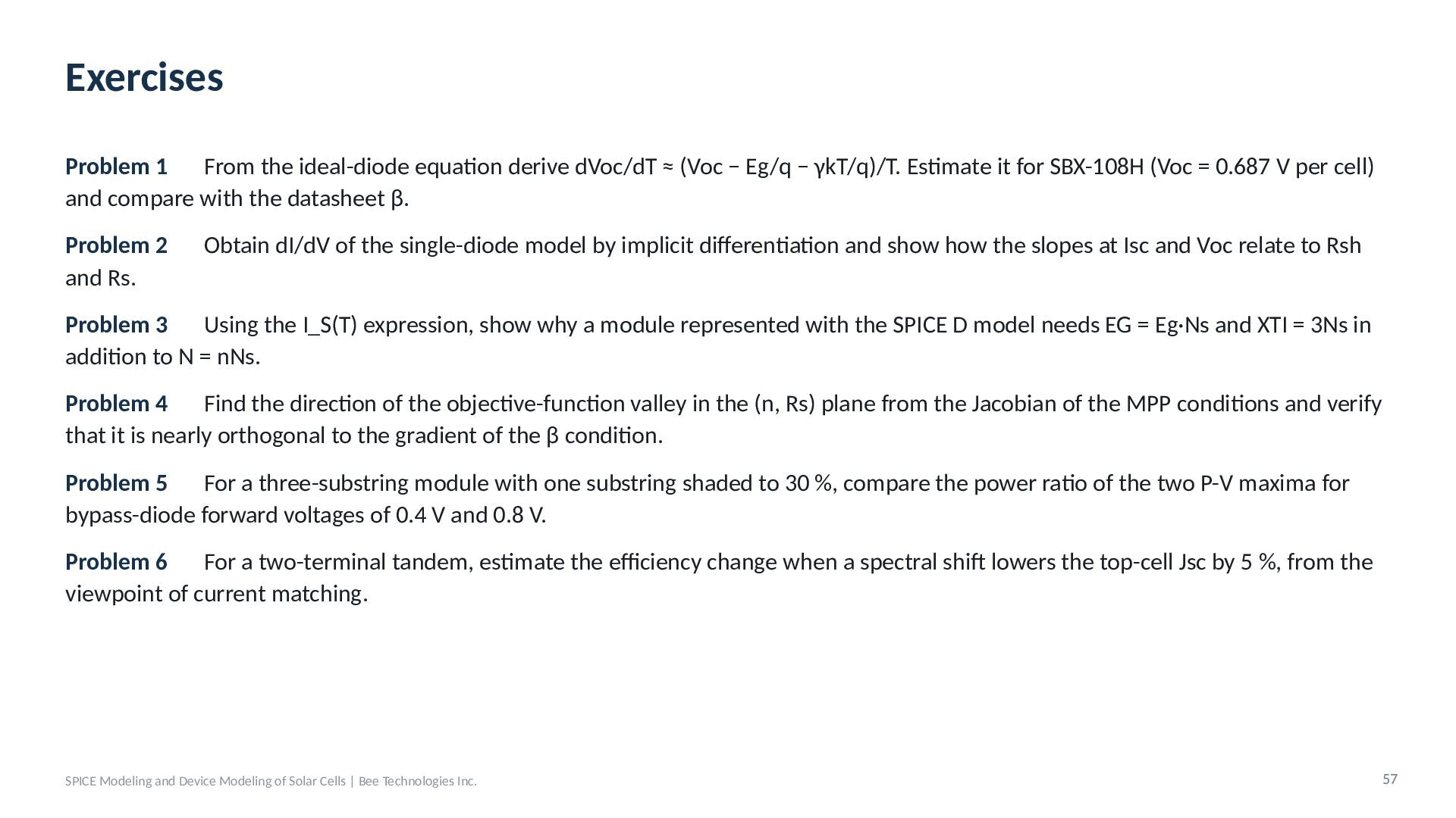
57. Exercises Problem 1 From the ideal-diode equation derive dVoc/dT ≈ (Voc − Eg/q − γkT/q)/T. Estimate it for SBX-108H (Voc = 0.687 V per cell) and compare with the datasheet β. Problem 2 and Rs. Obtain dI/dV of the single-diode model by implicit differentiation and show how the slopes at Isc and Voc relate to Rsh Problem 3 Using the I_S(T) expression, show why a module represented with the SPICE D model needs EG = Eg·Ns and XTI = 3Ns in addition to N = nNs. Problem 4 Find the direction of the objective-function valley in the (n, Rs) plane from the Jacobian of the MPP conditions and verify that it is nearly orthogonal to the gradient of the β condition. Problem 5 For a three-substring module with one substring shaded to 30 %, compare the power ratio of the two P-V maxima for bypass-diode forward voltages of 0.4 V and 0.8 V. Problem 6 For a two-terminal tandem, estimate the efficiency change when a spectral shift lowers the top-cell Jsc by 5 %, from the viewpoint of current matching. SPICE Modeling and Device Modeling of Solar Cells | Bee Technologies Inc. 57
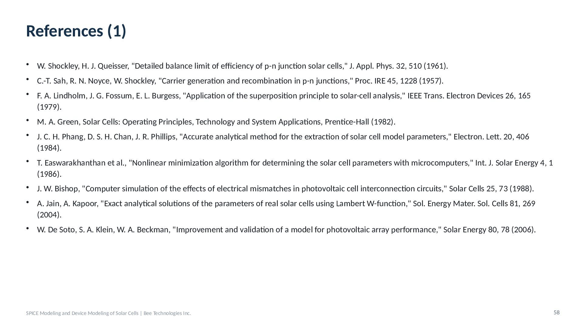
58. References (1) • W. Shockley, H. J. Queisser, "Detailed balance limit of efficiency of p-n junction solar cells," J. Appl. Phys. 32, 510 (1961). • C.-T. Sah, R. N. Noyce, W. Shockley, "Carrier generation and recombination in p-n junctions," Proc. IRE 45, 1228 (1957). • F. A. Lindholm, J. G. Fossum, E. L. Burgess, "Application of the superposition principle to solar-cell analysis," IEEE Trans. Electron Devices 26, 165 (1979). • M. A. Green, Solar Cells: Operating Principles, Technology and System Applications, Prentice-Hall (1982). • J. C. H. Phang, D. S. H. Chan, J. R. Phillips, "Accurate analytical method for the extraction of solar cell model parameters," Electron. Lett. 20, 406 (1984). • T. Easwarakhanthan et al., "Nonlinear minimization algorithm for determining the solar cell parameters with microcomputers," Int. J. Solar Energy 4, 1 (1986). • J. W. Bishop, "Computer simulation of the effects of electrical mismatches in photovoltaic cell interconnection circuits," Solar Cells 25, 73 (1988). • A. Jain, A. Kapoor, "Exact analytical solutions of the parameters of real solar cells using Lambert W-function," Sol. Energy Mater. Sol. Cells 81, 269 (2004). • W. De Soto, S. A. Klein, W. A. Beckman, "Improvement and validation of a model for photovoltaic array performance," Solar Energy 80, 78 (2006). SPICE Modeling and Device Modeling of Solar Cells | Bee Technologies Inc. 58
59. References (2) • L. Castañer, S. Silvestre, Modelling Photovoltaic Systems Using PSpice, Wiley (2002). • D. L. King, W. E. Boyson, J. A. Kratochvil, "Photovoltaic array performance model," Sandia Report SAND2004-3535 (2004). • M. G. Villalva, J. R. Gazoli, E. R. Filho, "Comprehensive approach to modeling and simulation of photovoltaic arrays," IEEE Trans. Power Electron. 24, 1198 (2009). • K. Ishaque, Z. Salam, H. Taheri, "Simple, fast and accurate two-diode model for photovoltaic modules," Sol. Energy Mater. Sol. Cells 95, 586 (2011). • A. P. Dobos, "An improved coefficient calculator for the California Energy Commission 6 parameter photovoltaic module model," J. Sol. Energy Eng. 134, 021011 (2012). • A. Laudani, F. Riganti Fulginei, A. Salvini, "Identification of the one-diode model for photovoltaic modules from datasheet values," Solar Energy 108, 432 (2014). • D. Moia et al., "Ionic-to-electronic current amplification in hybrid perovskite solar cells," Energy Environ. Sci. 12, 1296 (2019). • W. F. Holmgren, C. W. Hansen, M. A. Mikofski, "pvlib python: a python package for modeling solar energy systems," J. Open Source Softw. 3, 884 (2018). • IEC 61215-1:2021, IEC 60891:2021, IEC TS 60904-1-2:2019 SPICE Modeling and Device Modeling of Solar Cells | Bee Technologies Inc. 59