lecture26.pdf

Transcript

1. Session 26 ICS 211 Hash Tables
2. Memory Upload • Terminology • Hash Functions • Collisions • Open Addressing • Restructuring the Hash Table • Efficiency of Hashing
3. Terminology • A table is an abstract data type that stores & retrieves records according to their search key values  Also called a dictionary  Record: each individual row in the table
4. Terminology • A table can be implemented in many ways  Array, linked list, binary search trees, …  For example, a binary search tree of tax records, where the SSN is the search key
5. Terminology • Hashing: a way to access a table in relatively constant (quick) time  Uses a hash function & collision resolution scheme
6. Terminology • Hash function: a mathematical calculation that maps the search key to an index in a hash table  Should be fast to calculate & distribute items evenly  Time for calculation should be O(1)
7. Terminology • Hash table: an array of table items, where the index is calculated by a hash function  Instead of having to search through the table, comparing the search key to the search key of each item, we can use a hash function on the search key to quickly calculate the index of the item
8. Terminology • 911 emergency system for Kaunakakai, Molokai (population 3,425)  Could store everyone’s records with name, address, and telephone number using telephone numbers as search key  Could use entire telephone number, but wastes too much space (10,000,000,000 array elements)
9. Terminology • 911 emergency system for Kaunakakai, Molokai (population 3,425)  Better to use last four digits of telephone number (10,000 array elements)  For example, use table[4567] rather than table[8081234567] to access records
10. Terminology • A hash function is written h(x)=i  h is the name of the function  x is the record search key  i is the location (index) in the hash table (typically an array)  Once i is calculated, then table[i] contains a reference to the corresponding record
11. Terminology • A hash function is written h(x)=i  In the 911 emergency system example: h(8081234567)=4567  table[4567] contains a reference to a record with the person’s name, address, and telephone number (the search key is the telephone number)
12. Example Hash Functions • Three simple hash functions for integers 1. Selecting digits 2. Folding 3. Modulus arithmetic
13. Example Hash Functions • Selecting digits hash function  Instead of using the whole integer, only select several digits  For example, if you have the SS#123-45-6789, just use the first 3 digits  h(123456789) = 123
14. Example Hash Functions • Selecting digits hash function  Fast & easy to calculate, but usually does not distribute randomly  The first three numbers of a social security number are based on location, so people of the same state usually have the same first three numbers for the SS#
15. Example Hash Functions • Folding hash function  Add the digits of the integer together  For example, if you have the SS#123- 45-6789, add all the digits together  h(123456789)=1+2+3+4+5+6+7+8+9 =45 with hash table index range 0 < h(search key) < 81
16. Example Hash Functions • Folding hash function  Can add in different ways to adjust to hash tables of different sizes (different index ranges)  h(123456789)=123+456+789=1368 with hash table index range 0 < h(search key) < 2997
17. Example Hash Functions • Modulus arithmetic hash function  Using modulus as a hash function  h(x) = x mod tableSize  Modulus (mod or % ) is the remainder of a division
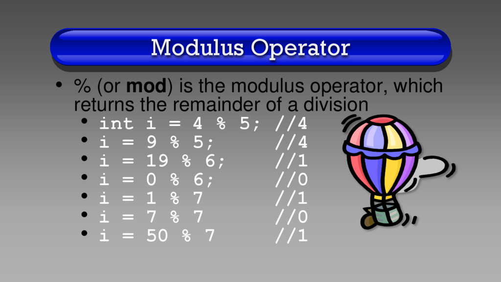
18. Modulus Operator • % (or mod) is the modulus operator, which returns the remainder of a division • int i = 4 % 5; //4 • i = 9 % 5; //4 • i = 19 % 6; //1 • i = 0 % 6; //0 • i = 1 % 7 //1 • i = 7 % 7 //0 • i = 50 % 7 //1
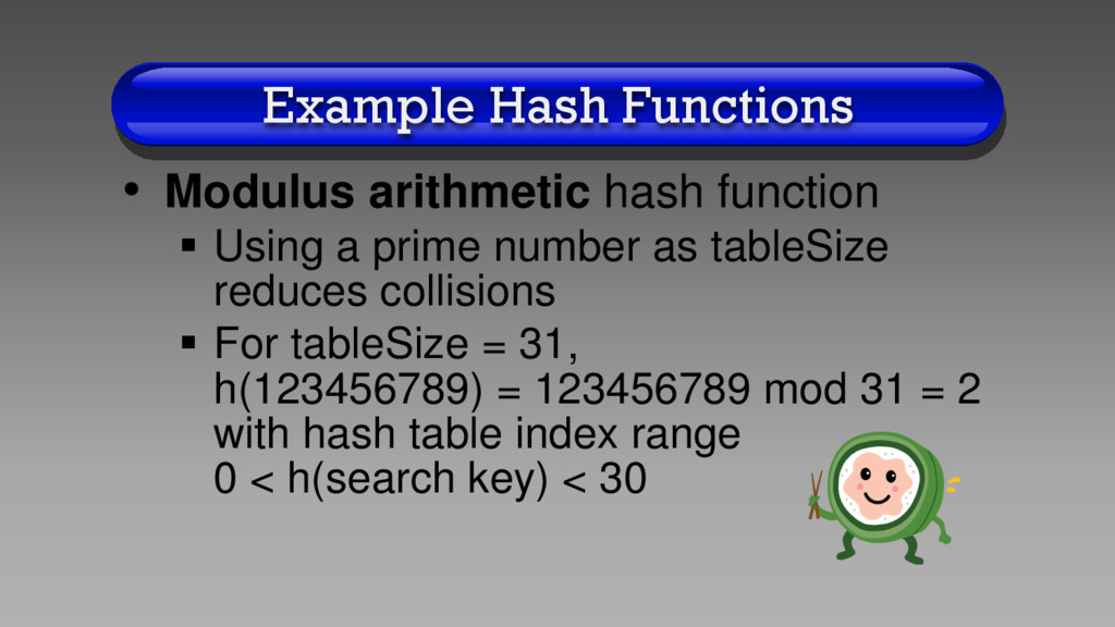
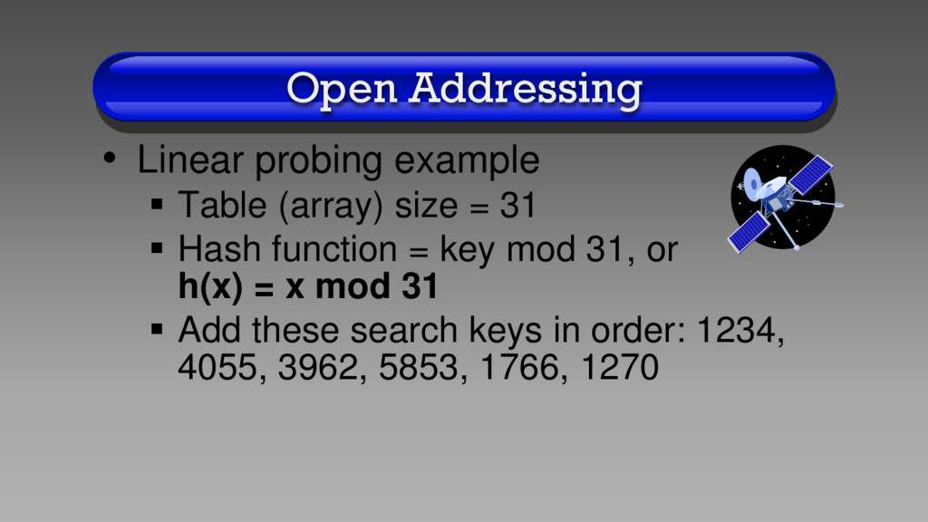
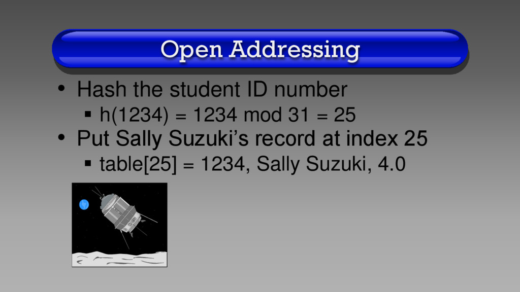
19. Example Hash Functions • Modulus arithmetic hash function  Using a prime number as tableSize reduces collisions  For tableSize = 31, h(123456789) = 123456789 mod 31 = 2 with hash table index range 0 < h(search key) < 30
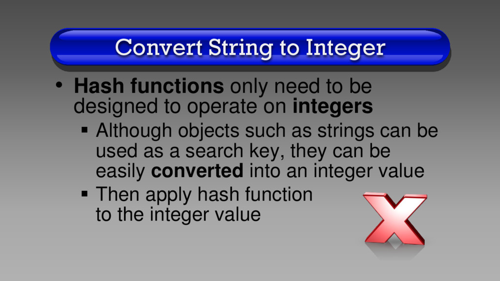
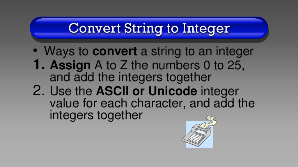
20. Convert String to Integer • Hash functions only need to be designed to operate on integers  Although objects such as strings can be used as a search key, they can be easily converted into an integer value  Then apply hash function to the integer value
21. Convert String to Integer • Ways to convert a string to an integer 1. Assign A to Z the numbers 0 to 25, and add the integers together 2. Use the ASCII or Unicode integer value for each character, and add the integers together
22. Convert String to Integer • Ways to convert a string to an integer 3. Use the binary number for the ASCII or Unicode integer value for each character, and concatenate the binary numbers together
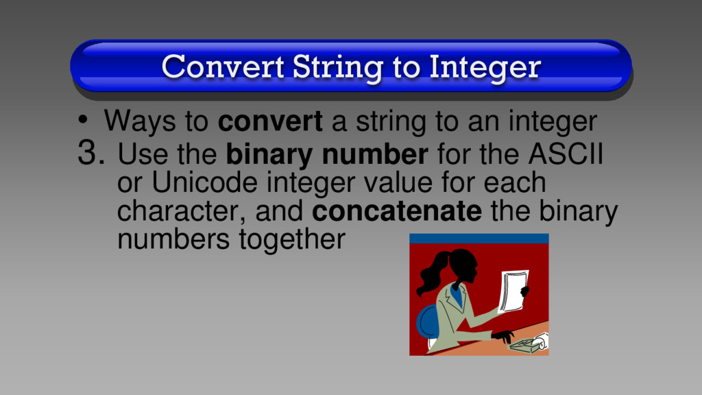
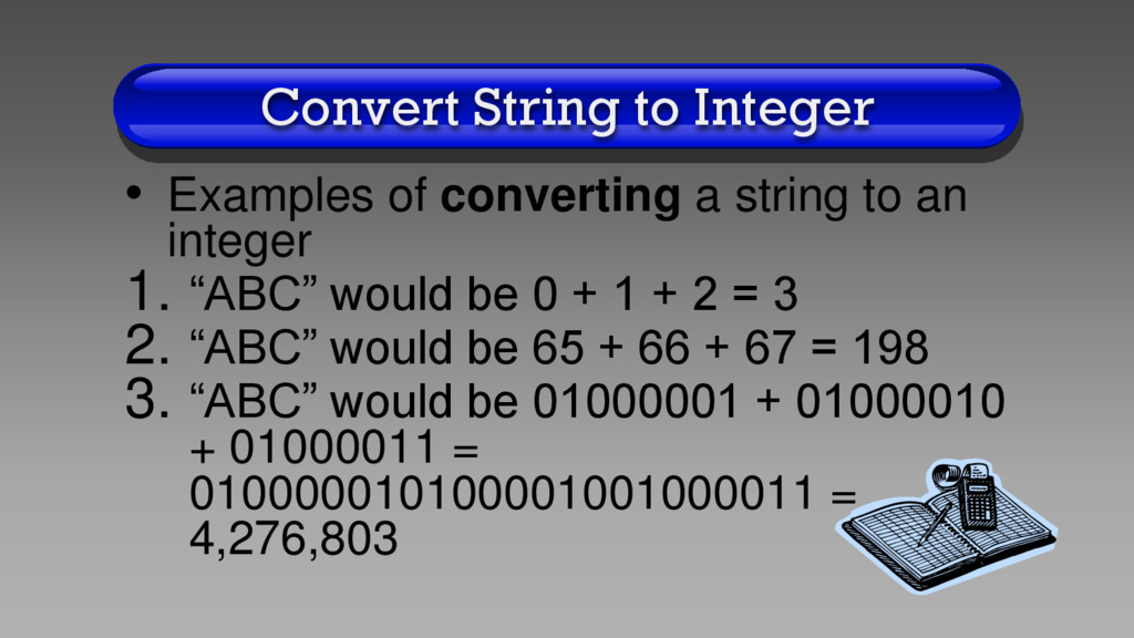
23. Convert String to Integer • Examples of converting a string to an integer 1. “ABC” would be 0 + 1 + 2 = 3 2. “ABC” would be 65 + 66 + 67 = 198 3. “ABC” would be 01000001 + 01000010 + 01000011 = 010000010100001001000011 = 4,276,803
24. Java Hash Function • All Java API classes have a hash function already defined!  For example, check out class String  See the public int hashCode() method  Returns a hash code for this string
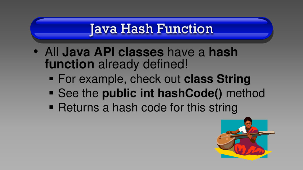
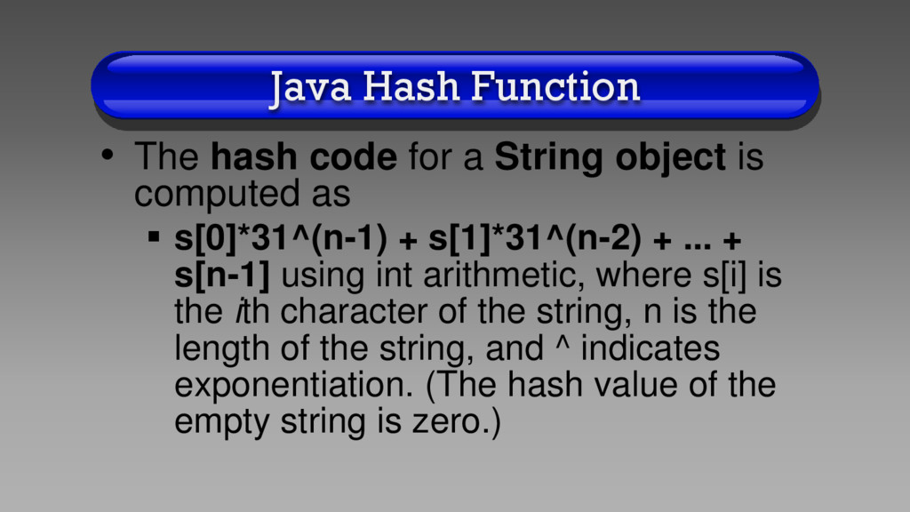
25. Java Hash Function • The hash code for a String object is computed as  s[0]*31^(n-1) + s[1]*31^(n-2) + ... + s[n-1] using int arithmetic, where s[i] is the ith character of the string, n is the length of the string, and ^ indicates exponentiation. (The hash value of the empty string is zero.)
26. Terminology • Perfect hash function  Ideal situation where hash function maps each search key into a different location in the hash table  For example, telephone numbers all map to different indexes
27. Terminology • Collision: when a hash function maps two or more search keys into the same location in the hash table • h(key1) = h(key2), so have the same index value
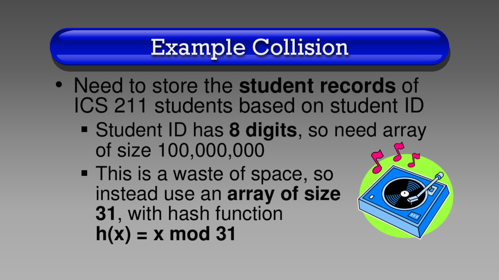
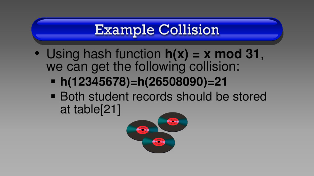
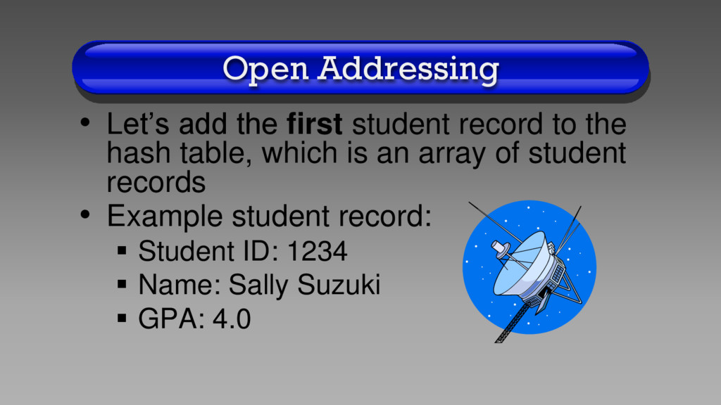
28. Example Collision • Need to store the student records of ICS 211 students based on student ID  Student ID has 8 digits, so need array of size 100,000,000  This is a waste of space, so instead use an array of size 31, with hash function h(x) = x mod 31
29. Example Collision • Using hash function h(x) = x mod 31, we can get the following collision:  h(12345678)=h(26508090)=21  Both student records should be stored at table[21]
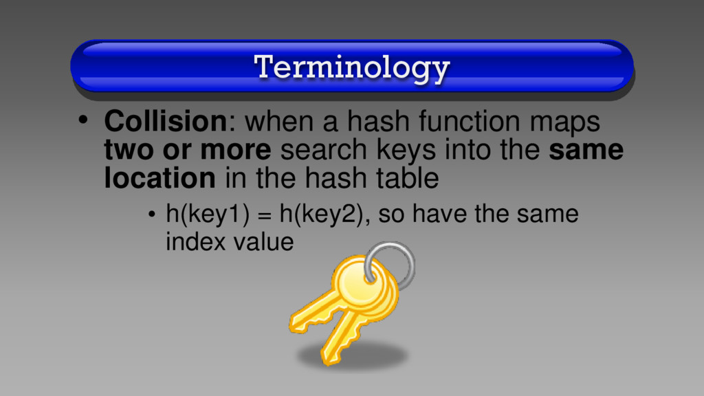
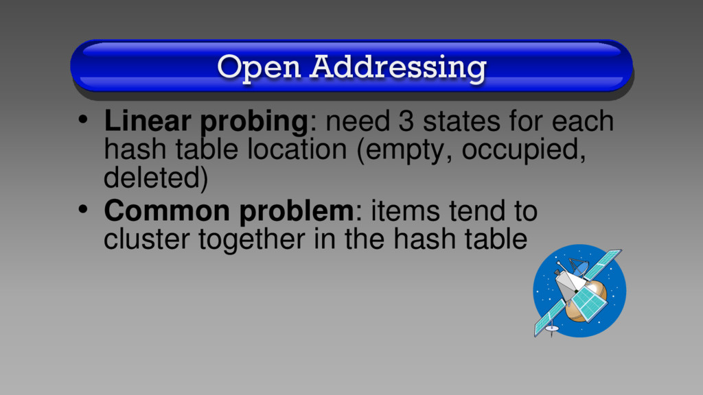
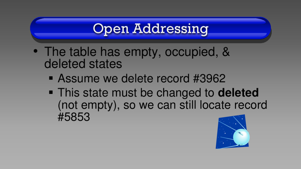
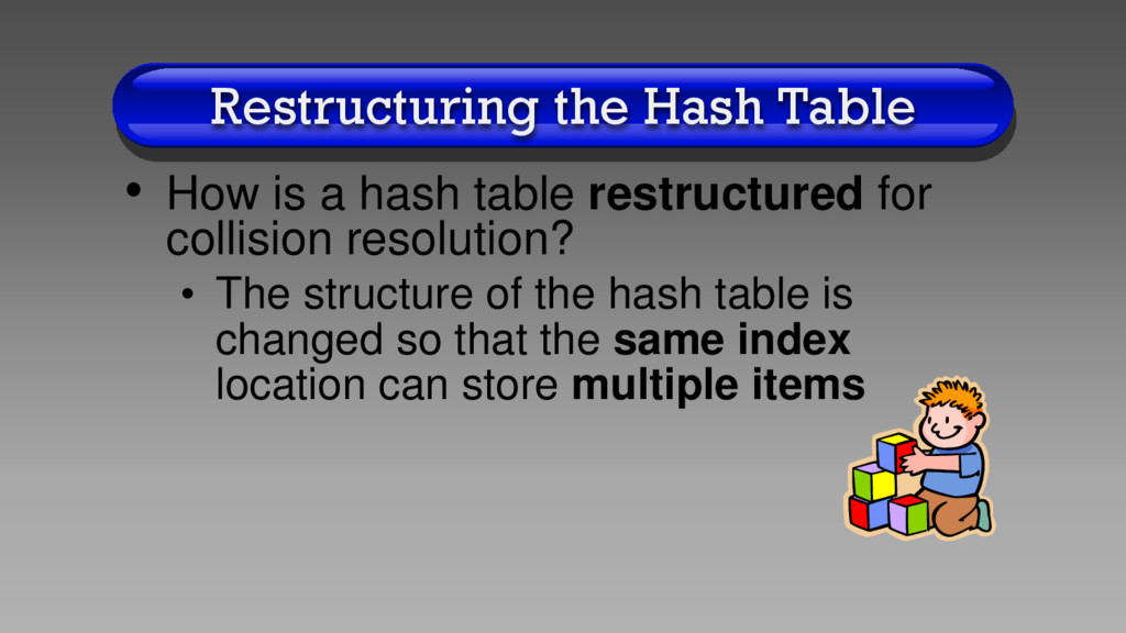
30. Collision Resolution • In case of a collision, a collision resolution scheme must be implemented • Collision resolution: assigns the search keys with the same hash function to different locations in the hash table
31. Collision Resolution • Collision resolution: whenever possible, items should be placed evenly in the hash table in order to avoid these collisions • Two main approaches to collision resolution 1. Open addressing 2. Restructure the hash table
32. Open Addressing • Open addressing: probe (search) for open locations in the hash table • Probe sequence: the sequence of locations that are examined for a possible open location to put the next item
33. Open Addressing • Three types of probing 1. Linear probing 2. Quadratic probing 3. Double hashing
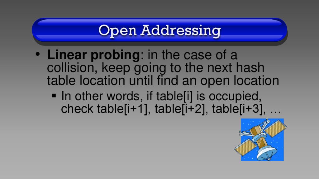
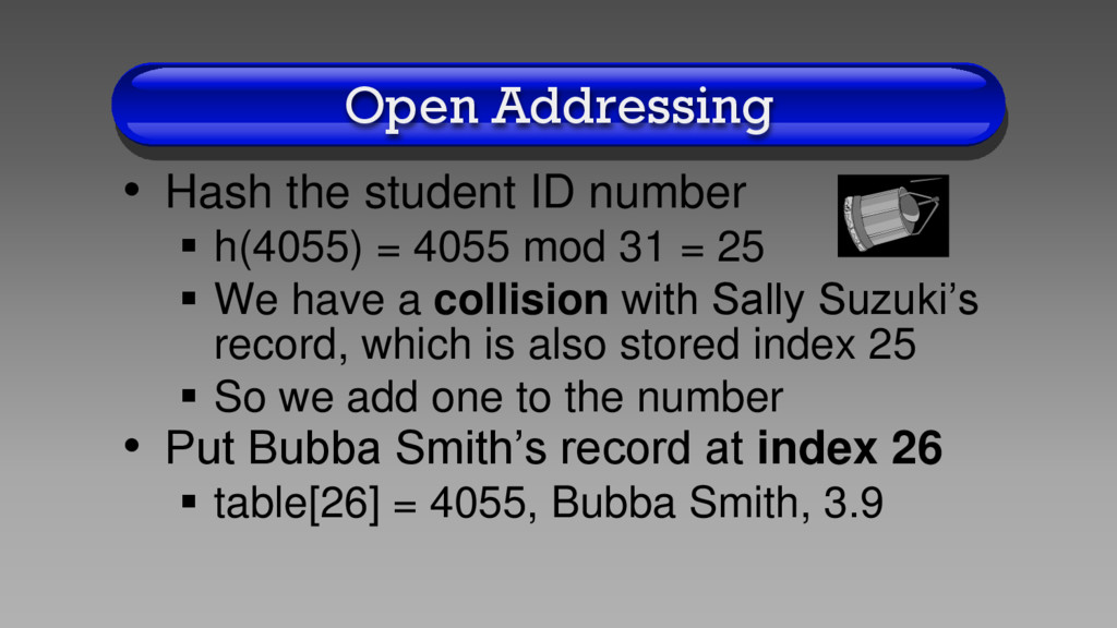
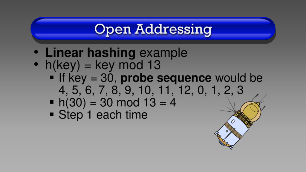
34. Open Addressing • Linear probing: in the case of a collision, keep going to the next hash table location until find an open location  In other words, if table[i] is occupied, check table[i+1], table[i+2], table[i+3], …
35. Open Addressing • Linear probing: need 3 states for each hash table location (empty, occupied, deleted) • Common problem: items tend to cluster together in the hash table
36. Open Addressing • Linear probing example  Table (array) size = 31  Hash function = key mod 31, or h(x) = x mod 31  Add these search keys in order: 1234, 4055, 3962, 5853, 1766, 1270
37. Open Addressing • Let’s add the first student record to the hash table, which is an array of student records • Example student record:  Student ID: 1234  Name: Sally Suzuki  GPA: 4.0
38. Open Addressing • Hash the student ID number  h(1234) = 1234 mod 31 = 25 • Put Sally Suzuki’s record at index 25  table[25] = 1234, Sally Suzuki, 4.0
39. Open Addressing • Let’s add the second student record to the hash table • Second student record:  Student ID: 4055  Name: Bubba Smith  GPA: 3.9
40. Open Addressing • Hash the student ID number  h(4055) = 4055 mod 31 = 25  We have a collision with Sally Suzuki’s record, which is also stored index 25  So we add one to the number • Put Bubba Smith’s record at index 26  table[26] = 4055, Bubba Smith, 3.9
41. Open Addressing • h(1234) = 25 table[25] = 1234 • h(4055) = 25+1 table[26] = 4055 • h(3962) = 25+2 table[27] = 3962 • h(5853) = 25+3 table[28] = 5853 • h(1766) = 30 table[30] = 1766 • h(1270) = 30+1 table[0] = 1270 (wraps around) • All other table entries are empty
42. Open Addressing • The table has empty, occupied, & deleted states  Assume we delete record #3962  This state must be changed to deleted (not empty), so we can still locate record #5853
43. Open Addressing • h(1234) = 25 table[25] = 1234 • h(4055) = 25+1 table[26] = 4055 • delete(3962) table[27] = “deleted” • h(5853) = 25+3 table[28] = 5853 • No record added table[29] = “empty” • h(1766) = 30 table[30] = 1766 • h(1270) = 30+1 table[0] = 1270 (wraps around)
44. Open Addressing • Linear hashing example • h(key) = key mod 13  If key = 30, probe sequence would be 4, 5, 6, 7, 8, 9, 10, 11, 12, 0, 1, 2, 3  h(30) = 30 mod 13 = 4  Step 1 each time
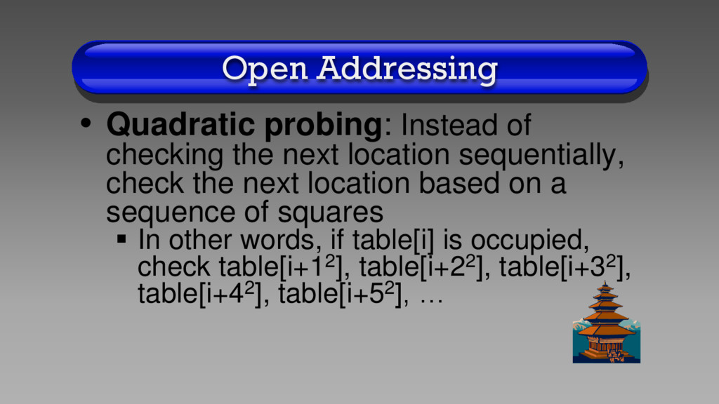
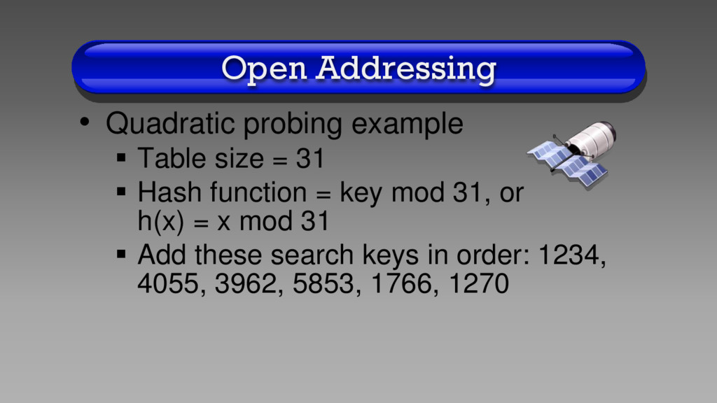
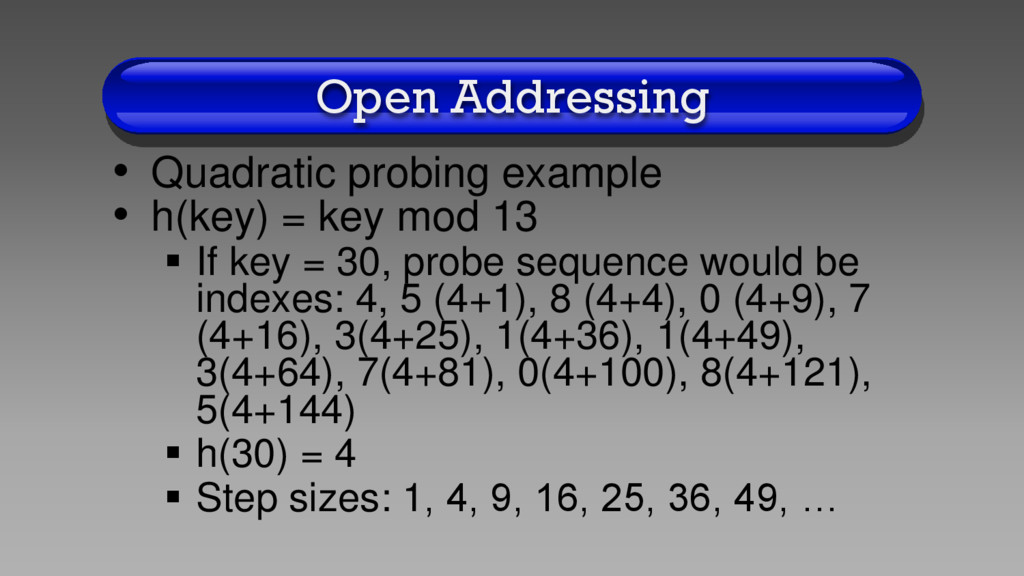
45. Open Addressing • Quadratic probing: Instead of checking the next location sequentially, check the next location based on a sequence of squares  In other words, if table[i] is occupied, check table[i+12], table[i+22], table[i+32], table[i+42], table[i+52], …
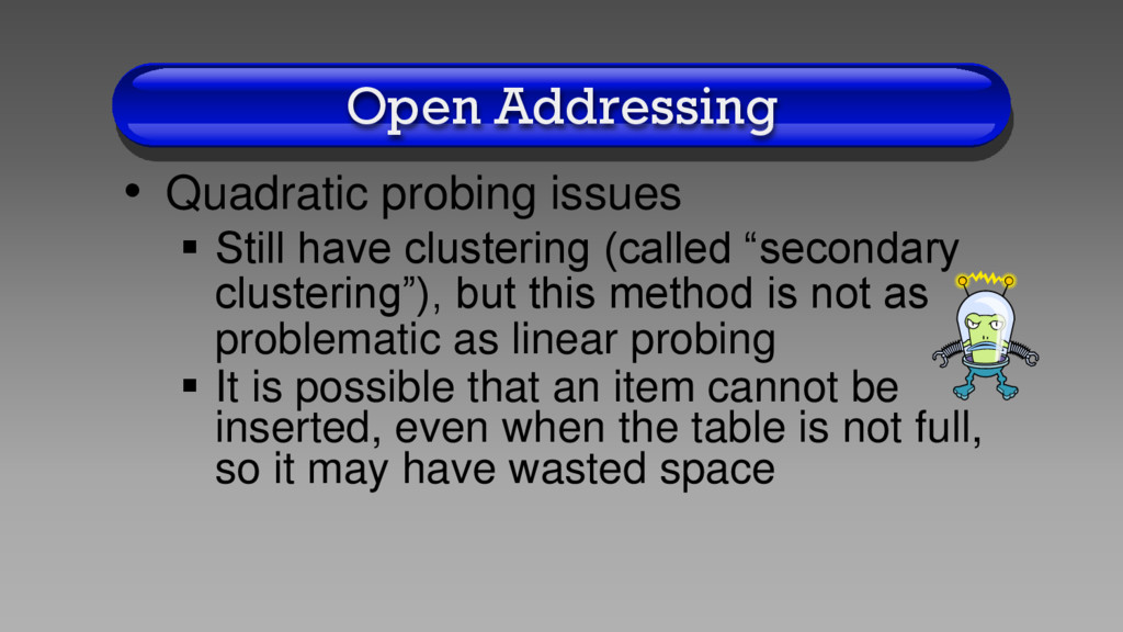
46. Open Addressing • Quadratic probing issues  Still have clustering (called “secondary clustering”), but this method is not as problematic as linear probing  It is possible that an item cannot be inserted, even when the table is not full, so it may have wasted space
47. Open Addressing • Quadratic probing example  Table size = 31  Hash function = key mod 31, or h(x) = x mod 31  Add these search keys in order: 1234, 4055, 3962, 5853, 1766, 1270
48. Open Addressing • h(1234) = 25 table[25] = 1234 • h(4055) = 25+12 table[26] = 4055 • h(3962) = 25+22 table[29] = 3962 • h(5853) = 25+32 table[3] = 5853 (wraps around) • h(1766) = 30 table[30] = 1766 • h(1270) = 30+12 table[0] = 1270 (wraps around)
49. Open Addressing • Quadratic probing example • h(key) = key mod 13  If key = 30, probe sequence would be indexes: 4, 5 (4+1), 8 (4+4), 0 (4+9), 7 (4+16), 3(4+25), 1(4+36), 1(4+49), 3(4+64), 7(4+81), 0(4+100), 8(4+121), 5(4+144)  h(30) = 4  Step sizes: 1, 4, 9, 16, 25, 36, 49, …
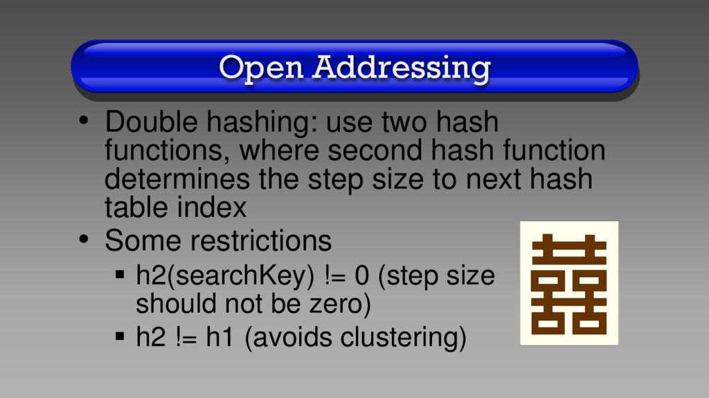
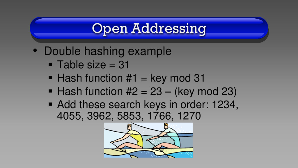
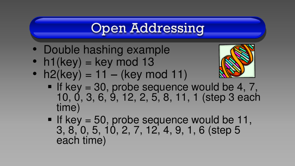
50. Open Addressing • Double hashing: use two hash functions, where second hash function determines the step size to next hash table index • Some restrictions  h2(searchKey) != 0 (step size should not be zero)  h2 != h1 (avoids clustering)
51. Open Addressing • Double hashing example  Table size = 31  Hash function #1 = key mod 31  Hash function #2 = 23 – (key mod 23)  Add these search keys in order: 1234, 4055, 3962, 5853, 1766, 1270
52. Open Addressing • h1(1234) = 25 table[25] = 1234 • h1(4055) = 25, h2(4055) = 16 (+25) table[10] = 4055 • h1(3962) = 25, h2(3962) = 17 (+25) table[11] = 3962 • h1(5853) = 25, h2(5853) = 12 (+25) table[6] = 5853
53. Open Addressing • h1(1766) = 30 table[30] = 1766 • h1(1270) = 30, h2(1270) = 18 (+30) table[17] = 1270 • All other table entries are empty
54. Open Addressing • Double hashing example • h1(key) = key mod 13 • h2(key) = 11 – (key mod 11)  If key = 30, probe sequence would be 4, 7, 10, 0, 3, 6, 9, 12, 2, 5, 8, 11, 1 (step 3 each time)  If key = 50, probe sequence would be 11, 3, 8, 0, 5, 10, 2, 7, 12, 4, 9, 1, 6 (step 5 each time)
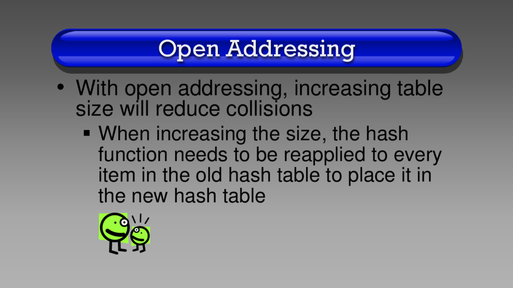
55. Open Addressing • With open addressing, increasing table size will reduce collisions  When increasing the size, the hash function needs to be reapplied to every item in the old hash table to place it in the new hash table
56. Restructuring the Hash Table • How is a hash table restructured for collision resolution? • The structure of the hash table is changed so that the same index location can store multiple items
57. Restructuring the Hash Table • Two ways to restructure a hash table for collision resolution: 1. Bucket hashing 2. Separate chaining
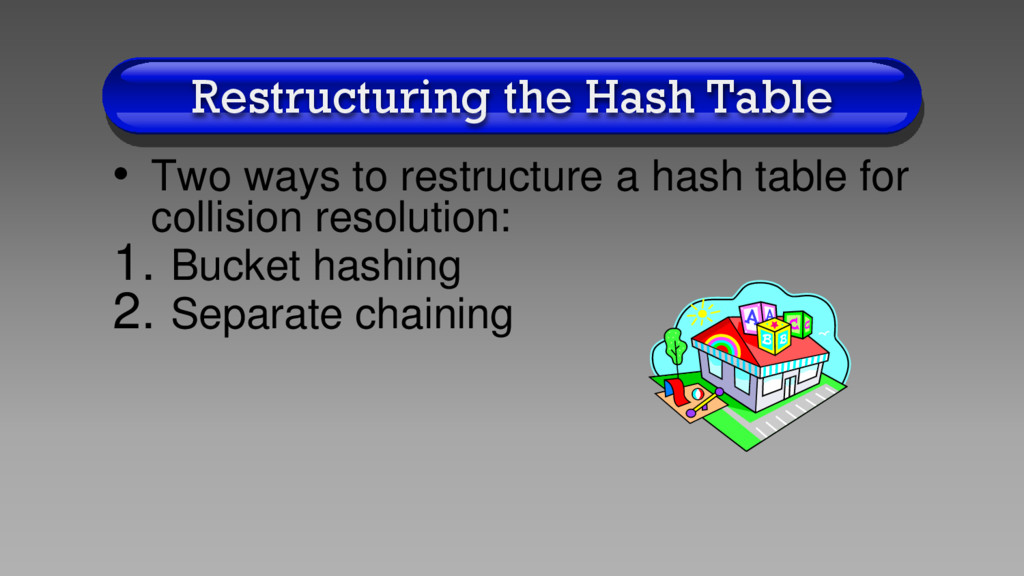
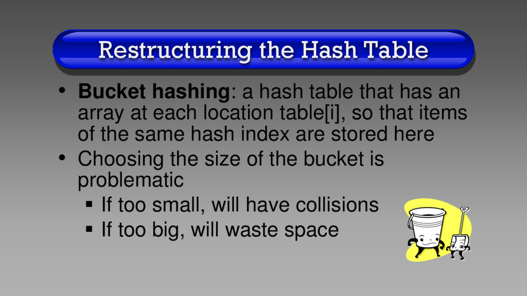
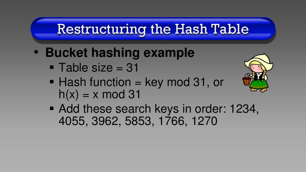
58. Restructuring the Hash Table • Bucket hashing: a hash table that has an array at each location table[i], so that items of the same hash index are stored here • Choosing the size of the bucket is problematic  If too small, will have collisions  If too big, will waste space
59. Restructuring the Hash Table • Bucket hashing example  Table size = 31  Hash function = key mod 31, or h(x) = x mod 31  Add these search keys in order: 1234, 4055, 3962, 5853, 1766, 1270
60. Restructuring the Hash Table • h(1234) = 25 table[25][0] = 1234 • h(4055) = 25 table[25][1] = 4055 • h(3962) = 25 table[25][2] = 3962 • h(5853) = 25 table[25][3] = 5853 • h(1766) = 30 table[30][0] = 1766 • h(1270) = 30 table[30][1] = 1270 • All other table entries are empty
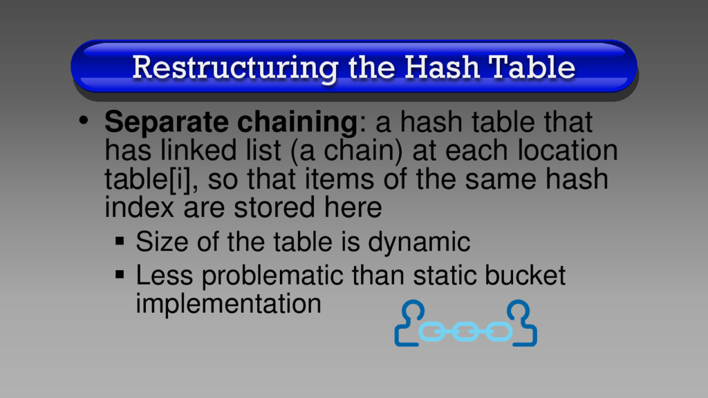
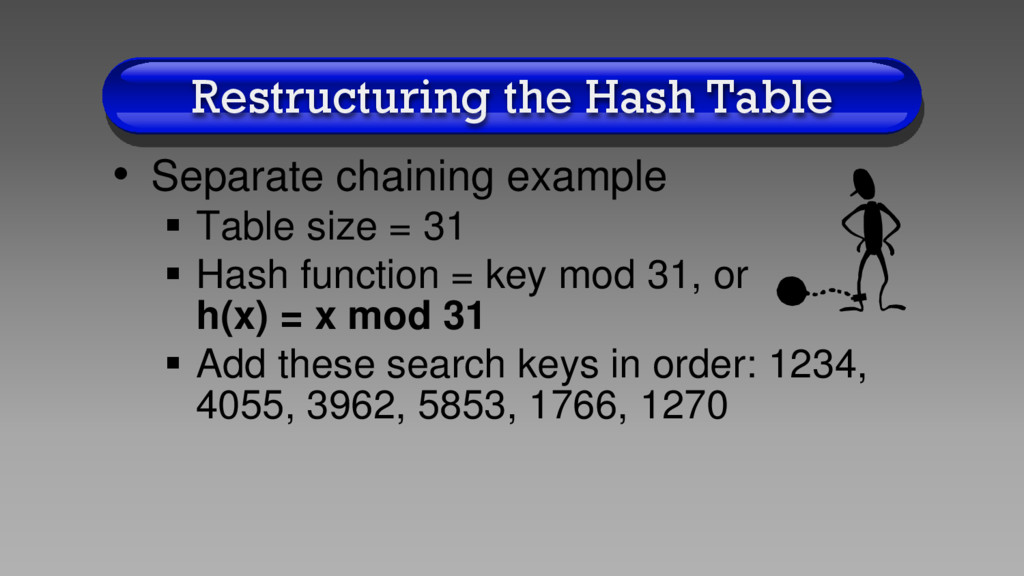
61. Restructuring the Hash Table • Separate chaining: a hash table that has linked list (a chain) at each location table[i], so that items of the same hash index are stored here  Size of the table is dynamic  Less problematic than static bucket implementation
62. Restructuring the Hash Table • Separate chaining example  Table size = 31  Hash function = key mod 31, or h(x) = x mod 31  Add these search keys in order: 1234, 4055, 3962, 5853, 1766, 1270
63. Restructuring the Hash Table • h(1234) = 25, table[25]=>1234 • h(4055) = 25, table[25]=>4055=>1234 • h(3962) = 25, table[25]=>3962=>4055=>1234 • h(5853) = 25, table[25]=>5853=>3962=>4055=>1234 • h(1766) = 30, table[30]=>1766 • h(1270) = 30, table[30]=>1270=>1766
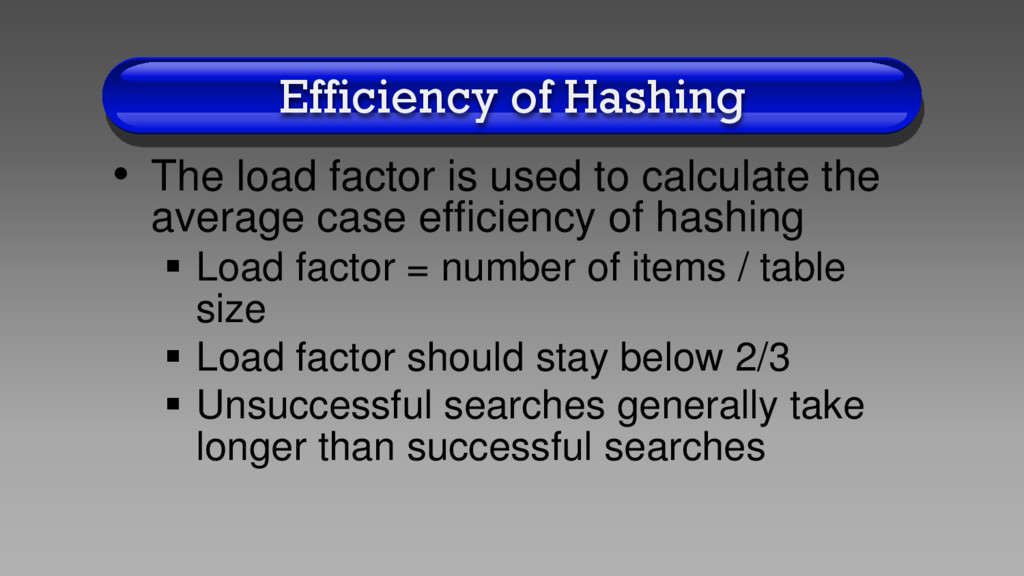
64. Efficiency of Hashing • The load factor is used to calculate the average case efficiency of hashing  Load factor = number of items / table size  Load factor should stay below 2/3  Unsuccessful searches generally take longer than successful searches
65. Efficiency of Hashing • Comparisons of implementations (slowest to quickest)  Linear probing > quadratic probing & double hashing > separate chaining
66. Memory Defragmenter • Terminology • Hash Functions • Collisions • Open Addressing • Restructuring the Hash Table • Efficiency of Hashing
67. Task Manager • Before the next class, you need to: 1.Do the assignment corresponding to this lecture 2.Email me any questions you may have about the material 3.Turn in the assignment before the next lecture 4.Be a slacker and go surfing!