SOC 4650 & SOC 5650 - Lecture 03

Slides for Lecture 03 of the Saint Louis University Course Introduction to GIS. These slides introduce data cleaning and wrangling processes.

Transcript

1. Install the janitor and naniar packages in R Please sit in the same place you sat last night! WELCOME! GETTING STARTED Check Slack’s #_news channel for a link to this week’s entry ticket
2. THE NATURE OF SPATIAL DATA (PART 1) INTRO TO GISC CHRISTOPHER PRENER, PH.D. SPRING, 2018 WEEK 04 LECTURE 03
3. AGENDA INTRO TO GISC / WEEK 04 / LECTURE 03 1. Front Matter 2. GISc & Public Policy 3. Types of Data 4. Methodological Challenges in GISc 5. Data Wrangling 6. Back Matter
4. 1 FRONT 
 MATTER
5. LP-04, Lab-02, and PS-01 are all due next class (February 12th) 1. FRONT MATTER ANNOUNCEMENTS Please sit at the same computer you worked at last class! We’ll be putting final project workgroups together this week.
6. GISC & PUBLIC POLICY 2
7. TYPES OF DATA 3
8. 3. TYPES OF DATA WHAT ARE SPATIAL DATA? Tabular Geometric
9. 3. TYPES OF DATA TABULAR DATA categorical ordinal continuous Tabular
10. 3. TYPES OF DATA TABULAR DATA categorical ordinal continuous crime “ucr crime type”
 1. murder 2. rape 3. robbery 4. aggravated assault
11. 3. TYPES OF DATA TABULAR DATA categorical ordinal continuous crimeStr “ucr crime type, string”
 murder rape robbery aggravated assault
12. 3. TYPES OF DATA TABULAR DATA categorical ordinal continuous newCrime “new incident”
 1. no 2. yes 0. 1.
13. 3. TYPES OF DATA TABULAR DATA qualitative ordinal continuous newCrime “new incident”
 1. no 2. yes 0. 1.
14. 3. TYPES OF DATA TABULAR DATA categorical ordinal continuous leadLevels “rate of exposure”
 1. very low 2. low 3. high 4. very high
15. 3. TYPES OF DATA TABULAR DATA categorical ordinal continuous leadCount “number of high tests”
 1 2 … 85
16. 3. TYPES OF DATA GEOMETRIC DATA Tabular Geometric
17. 3. TYPES OF DATA GEOMETRIC DATA Geometric Vector polygon Raster
18. 3. TYPES OF DATA GEOMETRIC DATA Vector point line polygon
19. 3. TYPES OF DATA GEOMETRIC DATA Vector point line polygon
20. 3. TYPES OF DATA GEOMETRIC DATA point line polygon
21. POINT GEOMETRIC DATA - SHAW CRIMES
22. 3. TYPES OF DATA GEOMETRIC DATA point line polygon zero dimensional data - 
 no length or width
23. 3. TYPES OF DATA GEOMETRIC DATA point line polygon
24. LINE GEOMETRIC DATA - STREET CENTERLINES
25. 3. TYPES OF DATA GEOMETRIC DATA point line polygon one dimensional data - 
 has length but not width
26. 3. TYPES OF DATA GEOMETRIC DATA point line polygon
27. POLYGON GEOMETRIC DATA - BUILDING FOOTPRINTS
28. 3. TYPES OF DATA GEOMETRIC DATA point line polygon two dimensional data - 
 has length and width
29. 3. TYPES OF DATA GEOMETRIC DATA Raster
30. RASTER GEOMETRIC DATA - SHAW CRIMES
31. RASTER GEOMETRIC DATA - SHAW CRIMES
32. METHODOLOGICAL CHALLENGES IN GISC 4
33. EVERYTHING IS RELATED TO EVERYTHING ELSE, BUT NEAR THINGS ARE MORE RELATED THAN DISTANT THINGS Waldo Tobler “A computer movie simulating 
 urban growth in the Detroit region”
 (1970)
34. 4. METHODOLOGICAL CHALLENGES IN GISC NEAR THINGS ARE LIKE OTHER NEAR THINGS Geographic patterning or “clustering” is referred to as spatial autocorrelation.
35. 4. METHODOLOGICAL CHALLENGES IN GISC NEAR THINGS ARE LIKE OTHER NEAR THINGS Geographic patterning or “clustering” is referred to as spatial autocorrelation. I = -1.000 I = 0.000 I = 0.857
36. 4. METHODOLOGICAL CHALLENGES IN GISC PAST BEHAVIOR IS PREDICTIVE When patterns repeat over time, like traveling the same route for your commute, we refer to them as having temporal autocorrelation.
37. THE SIERRA NEVADA 4. METHODOLOGICAL CHALLENGES IN GISC
38. THE SIERRA NEVADA 4. METHODOLOGICAL CHALLENGES IN GISC
39. KEY TERM Topographic maps are
 special types of reference
 maps that use a basemap with contour lines describing terrain - changes in the altitude and shape of the earth’s surface.
40. THE SIERRA NEVADA 4. METHODOLOGICAL CHALLENGES IN GISC
41. SPATIAL SAMPLING 4. METHODOLOGICAL CHALLENGES IN GISC
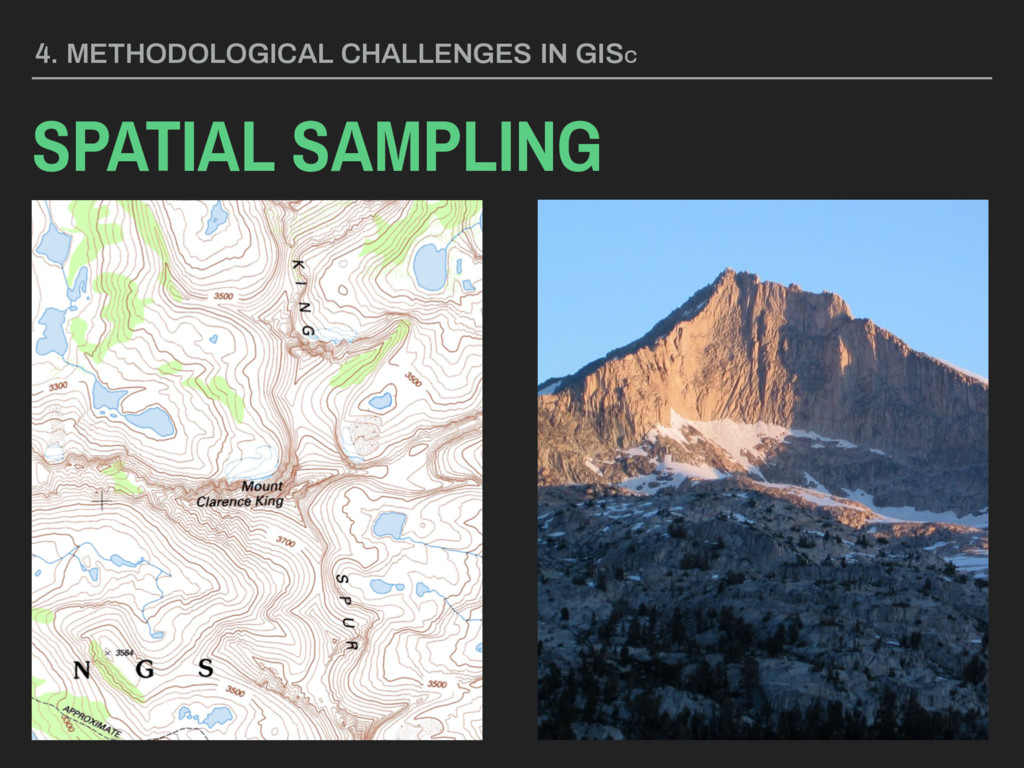
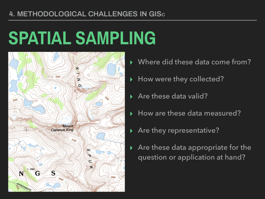
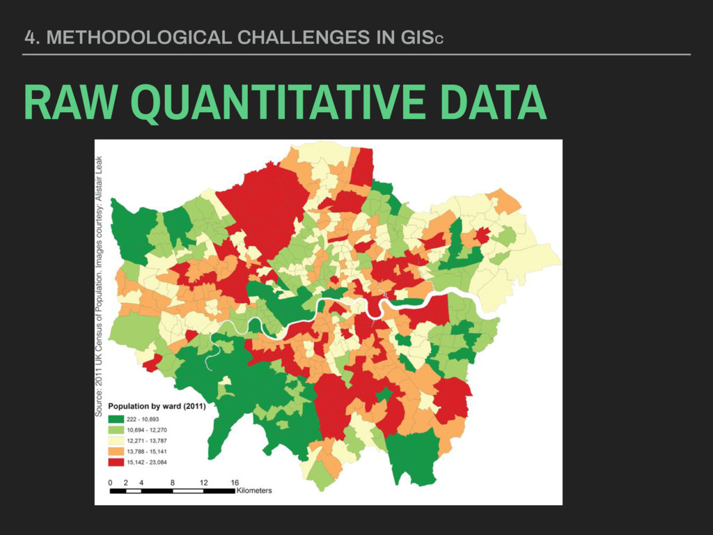
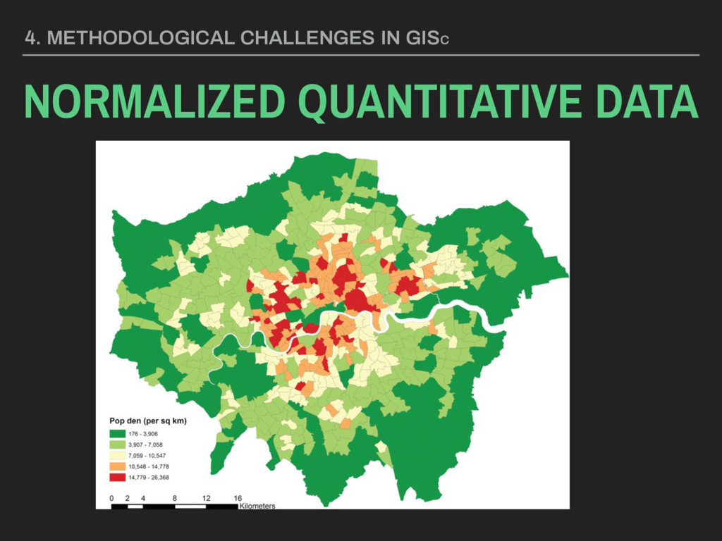
42. ▸ Where did these data come from? ▸ How were they collected? ▸ Are these data valid? ▸ How are these data measured? ▸ Are they representative? ▸ Are these data appropriate for the question or application at hand? 4. METHODOLOGICAL CHALLENGES IN GISC SPATIAL SAMPLING
43. THE MAINE COAST 4. METHODOLOGICAL CHALLENGES IN GISC
44. THE MAINE COAST 4. METHODOLOGICAL CHALLENGES IN GISC
45. THE MAINE COAST
46. SMALL SCALE Target Scale: 1:20,000,000
 Miles per Inch: ~316
47. LARGER SCALE Target Scale: 1:5,000,000
 Miles per Inch: ~79
48. LARGER SCALE Target Scale: 1:500,000
 Miles per Inch: ~7.89
49. SCALE & DISTANCE 1:20,000,000 1:500,000
50. SCALE & REPRESENTATION 1:20,000,000 1:500,000
51. LONDON 4. METHODOLOGICAL CHALLENGES IN GISC
52. RAW QUANTITATIVE DATA 4. METHODOLOGICAL CHALLENGES IN GISC
53. NORMALIZED QUANTITATIVE DATA 4. METHODOLOGICAL CHALLENGES IN GISC
54. DATA WRANGLING 5
55. 5. DATA WRANGLING HIGH LEVEL WORKFLOW 1. Plan 2. Organize 3. Document 4. Execute FOR EACH
 STEP:
56. IT IS OFTEN SAID THAT 80% OF DATA ANALYSIS IS SPENT ON THE PROCESS OF CLEANING AND PREPARING THE DATA Hadley Wickham “Tidy Data”
 (2014)
57. HAPPY FAMILIES ARE ALL ALIKE; EVERY UNHAPPY FAMILY IS UNHAPPY IN ITS OWN WAY Leo Tolstoy Anna Karenina
 (1878)
58. HAPPY FAMILIES ARE ALL ALIKE; EVERY UNHAPPY FAMILY IS UNHAPPY IN ITS OWN WAY Leo Tolstoy Anna Karenina
 (1878)
59. LIKE FAMILIES, TIDY DATASETS ARE ALL ALIKE BUT EVERY MESSY DATASET IS MESSY IN ITS OWN WAY. Hadley Wickham “Tidy Data”
 (2014)
60. TIDY DATASETS PROVIDE A STANDARDIZED WAY TO LINK THE STRUCTURE OF A DATASET (ITS PHYSICAL LAYOUT) WITH ITS SEMANTICS (ITS MEANING). Hadley Wickham “Tidy Data”
 (2014)
61. 5. DATA WRANGLING TIDY DATA Each variable should be saved in its own column. A B C D
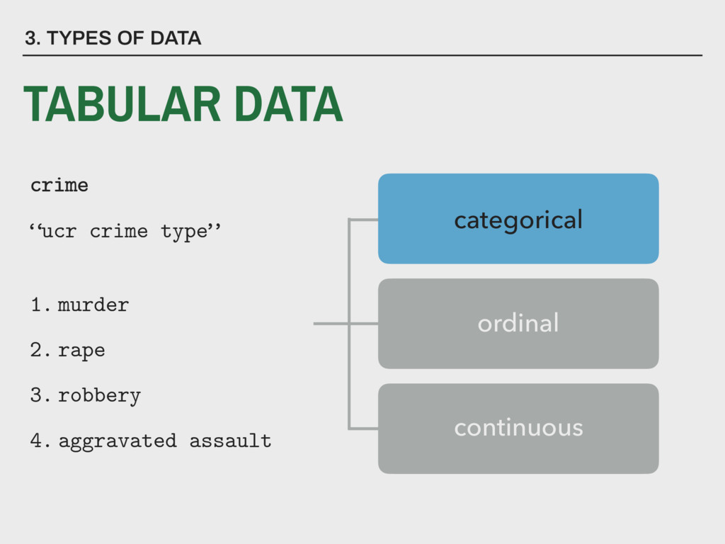
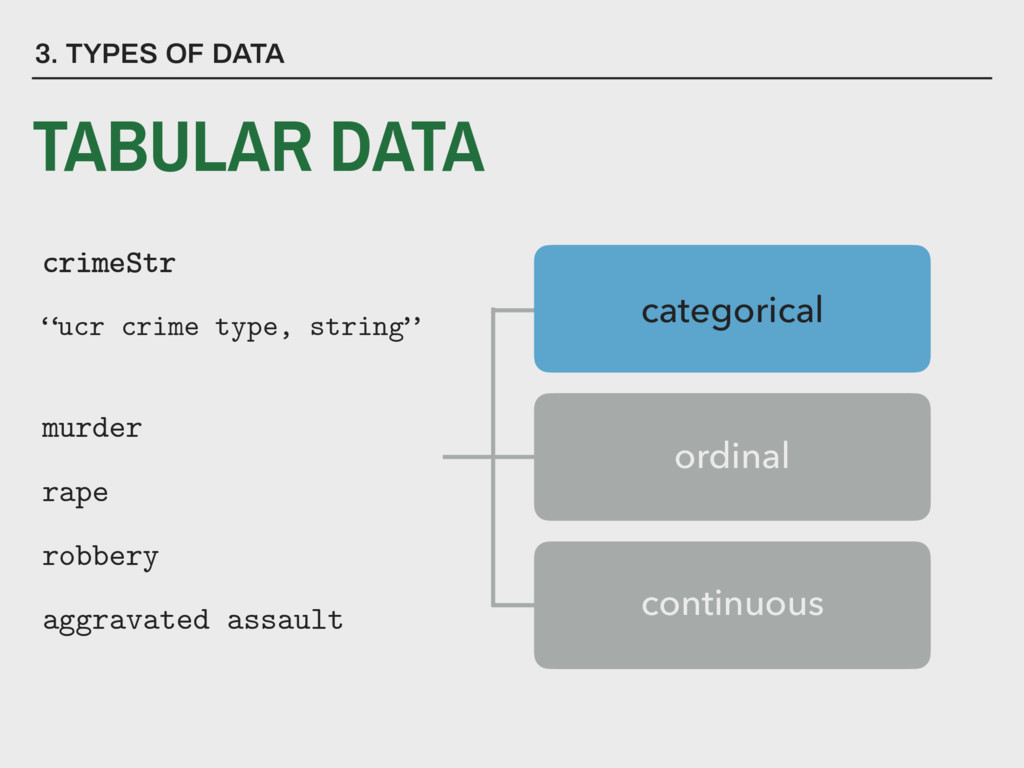
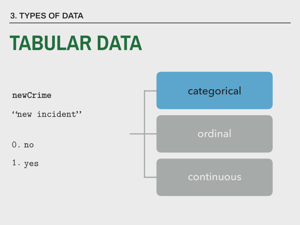
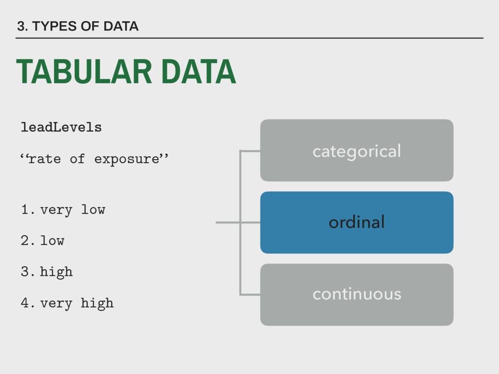
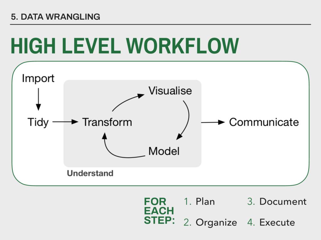
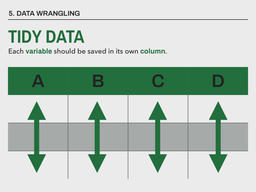
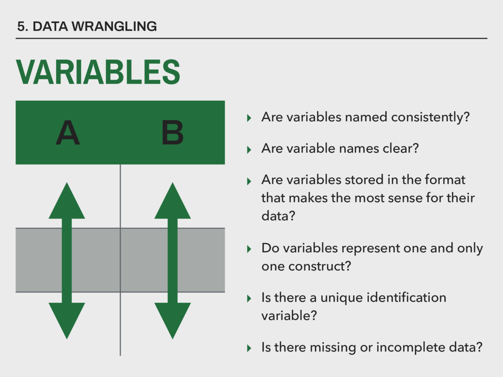
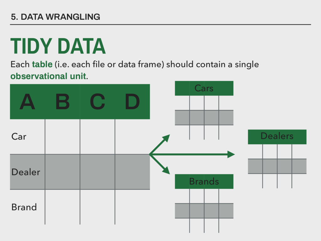
62. ▸ Are variables named consistently? ▸ Are variable names clear? ▸ Are variables stored in the format that makes the most sense for their data? ▸ Do variables represent one and only one construct? ▸ Is there a unique identification variable? ▸ Is there missing or incomplete data? 5. DATA WRANGLING A B VARIABLES
63. 5. DATA WRANGLING TIDY DATA Each observation should be saved in its own row. A B C D
64. ▸ What is the observational unit? 5. DATA WRANGLING A B OBSERVATIONS
65. 5. DATA WRANGLING TIDY DATA Each table (i.e. each file or data frame) should contain a single observational unit. A B C D Car Dealer Brand Cars Dealers Brands
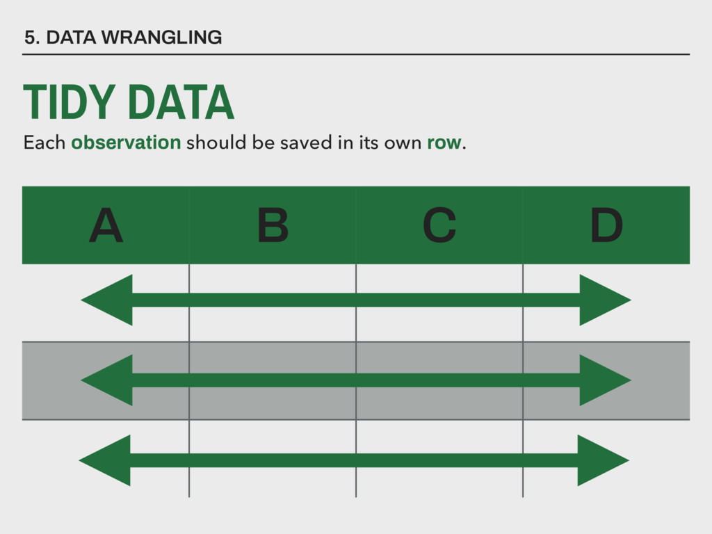
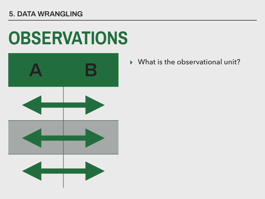
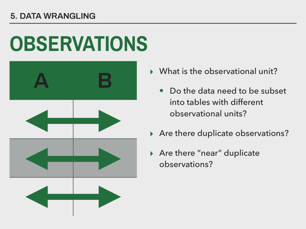
66. ▸ What is the observational unit? • Do the data need to be subset into tables with different observational units? ▸ Are there duplicate observations? ▸ Are there “near” duplicate observations? 5. DATA WRANGLING A B OBSERVATIONS
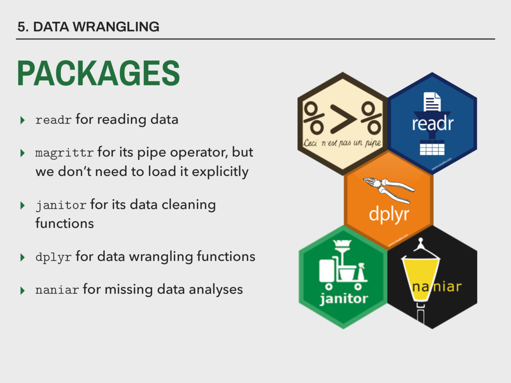
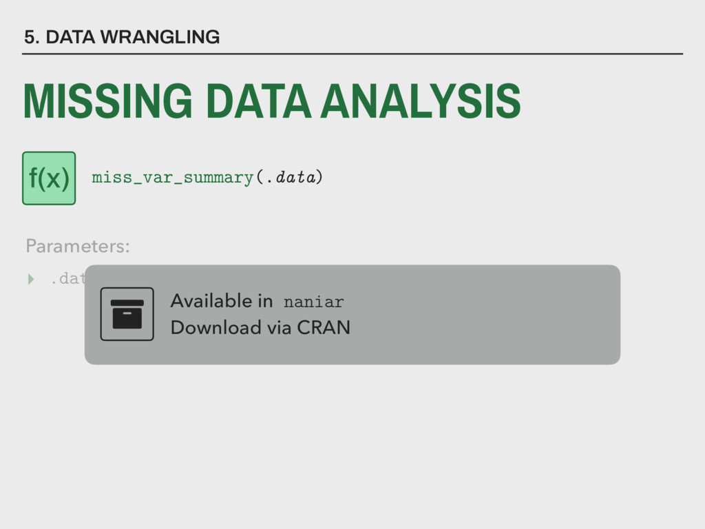
67. ▸ readr for reading data ▸ magrittr for its pipe operator, but we don’t need to load it explicitly ▸ janitor for its data cleaning functions ▸ dplyr for data wrangling functions ▸ naniar for missing data analyses 5. DATA WRANGLING PACKAGES
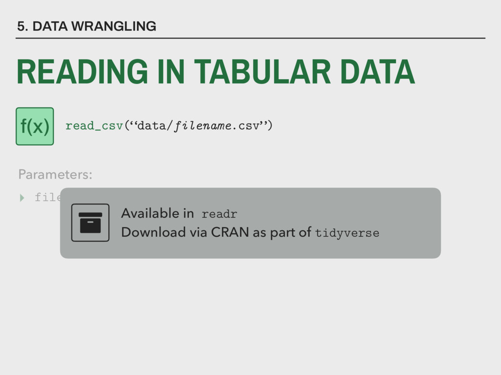
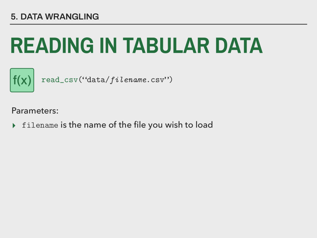
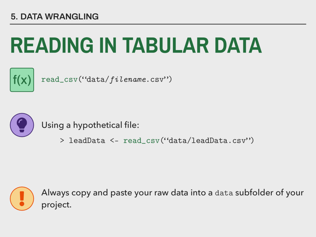
68. ▸ filename is the name of the file you wish to load Available in readr
 Download via CRAN as part of tidyverse 5. DATA WRANGLING READING IN TABULAR DATA Parameters: read_csv(“data/filename.csv”) f(x)
69. ▸ filename is the name of the file you wish to load 5. DATA WRANGLING READING IN TABULAR DATA Parameters: read_csv(“data/filename.csv”) f(x)
70. f(x) 5. DATA WRANGLING READING IN TABULAR DATA read_csv(“data/filename.csv”) Using a hypothetical file: > leadData <- read_csv(“data/leadData.csv”) Always copy and paste your raw data into a data subfolder of your project.
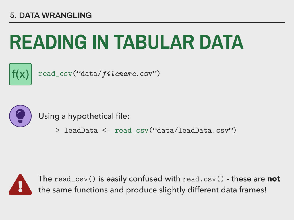
71. f(x) 5. DATA WRANGLING READING IN TABULAR DATA read_csv(“data/filename.csv”) Using a hypothetical file: > leadData <- read_csv(“data/leadData.csv”) The read_csv() is easily confused with read.csv() - these are not the same functions and produce slightly different data frames!
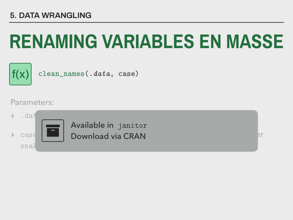
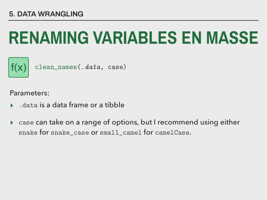
72. ▸ .data is a data frame or a tibble ▸ case can take on a range of options, but I recommend using either snake for snake_case or small_camel for camelCase. Available in janitor
 Download via CRAN 5. DATA WRANGLING RENAMING VARIABLES EN MASSE Parameters: clean_names(.data, case) f(x)
73. ▸ .data is a data frame or a tibble ▸ case can take on a range of options, but I recommend using either snake for snake_case or small_camel for camelCase. 5. DATA WRANGLING RENAMING VARIABLES EN MASSE Parameters: clean_names(.data, case) f(x)
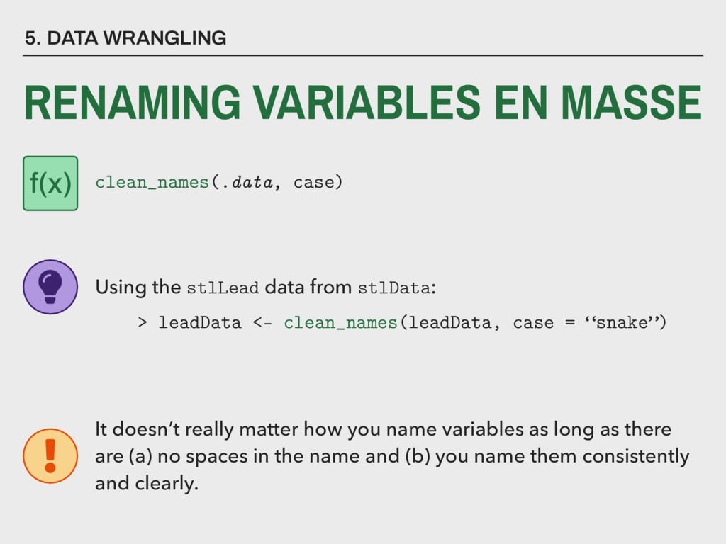
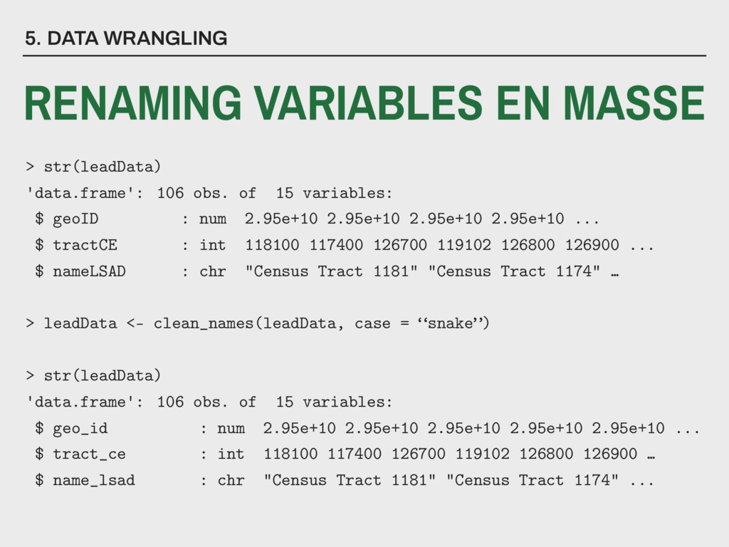
74. f(x) 5. DATA WRANGLING RENAMING VARIABLES EN MASSE clean_names(.data, case) Using the stlLead data from stlData: > leadData <- clean_names(leadData, case = “snake”) It doesn’t really matter how you name variables as long as there are (a) no spaces in the name and (b) you name them consistently and clearly.
75. 5. DATA WRANGLING RENAMING VARIABLES EN MASSE > str(leadData) 'data.frame': 106 obs. of 15 variables: $ geoID : num 2.95e+10 2.95e+10 2.95e+10 2.95e+10 ... $ tractCE : int 118100 117400 126700 119102 126800 126900 ... $ nameLSAD : chr "Census Tract 1181" "Census Tract 1174" … > leadData <- clean_names(leadData, case = “snake”) > str(leadData) 'data.frame': 106 obs. of 15 variables: $ geo_id : num 2.95e+10 2.95e+10 2.95e+10 2.95e+10 2.95e+10 ... $ tract_ce : int 118100 117400 126700 119102 126800 126900 … $ name_lsad : chr "Census Tract 1181" "Census Tract 1174" ...
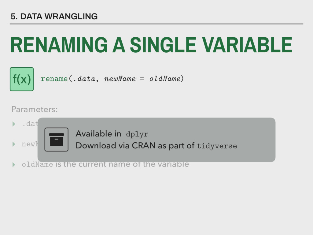
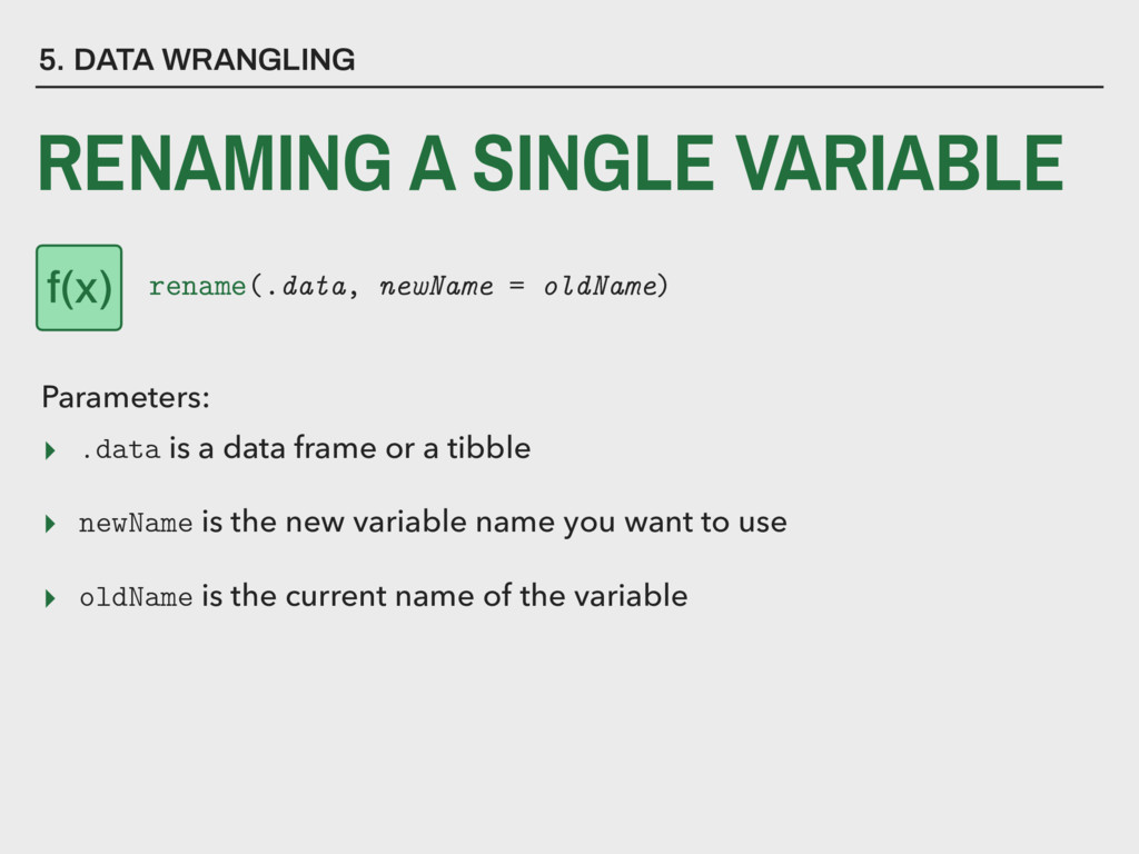
76. ▸ .data is a data frame or a tibble ▸ newName is the new variable name you want to use ▸ oldName is the current name of the variable Available in dplyr
 Download via CRAN as part of tidyverse 5. DATA WRANGLING RENAMING A SINGLE VARIABLE Parameters: rename(.data, newName = oldName) f(x)
77. ▸ .data is a data frame or a tibble ▸ newName is the new variable name you want to use ▸ oldName is the current name of the variable 5. DATA WRANGLING RENAMING A SINGLE VARIABLE Parameters: rename(.data, newName = oldName) f(x)
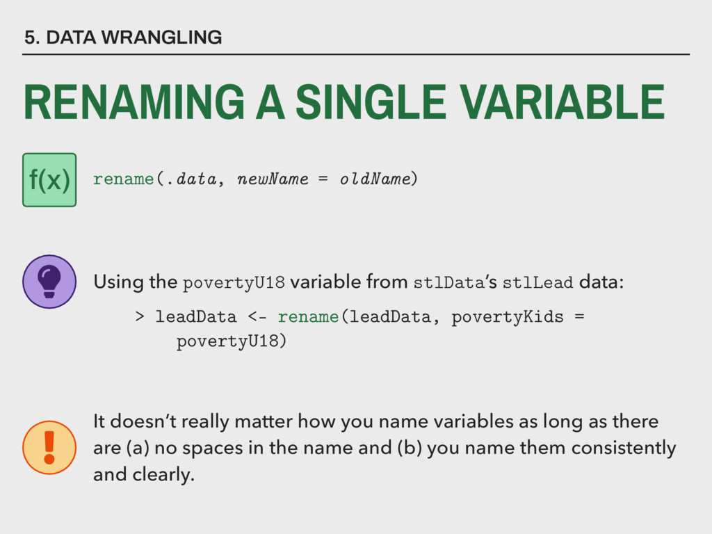
78. f(x) 5. DATA WRANGLING RENAMING A SINGLE VARIABLE rename(.data, newName = oldName) Using the povertyU18 variable from stlData’s stlLead data: > leadData <- rename(leadData, povertyKids = povertyU18) It doesn’t really matter how you name variables as long as there are (a) no spaces in the name and (b) you name them consistently and clearly.
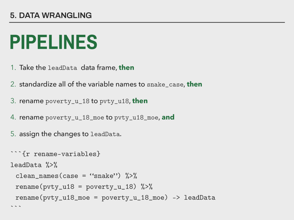
79. 5. DATA WRANGLING PIPELINES ```{r rename-variables} leadData %>% clean_names(case = “snake”) %>% rename(pvty_u18 = poverty_u_18) %>% rename(pvty_u18_moe = poverty_u_18_moe) -> leadData ``` 1. Take the leadData data frame, then 2. standardize all of the variable names to snake_case, then 3. rename poverty_u_18 to pvty_u18, then 4. rename poverty_u_18_moe to pvty_u18_moe, and 5. assign the changes to leadData.
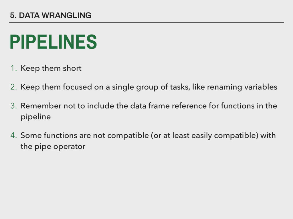
80. 5. DATA WRANGLING PIPELINES 1. Keep them short 2. Keep them focused on a single group of tasks, like renaming variables 3. Remember not to include the data frame reference for functions in the pipeline 4. Some functions are not compatible (or at least easily compatible) with the pipe operator
81. ▸ .data is a data frame or a tibble Available in naniar
 Download via CRAN 5. DATA WRANGLING MISSING DATA ANALYSIS Parameters: miss_var_summary(.data) f(x)
82. ▸ .data is a data frame or a tibble 5. DATA WRANGLING MISSING DATA ANALYSIS Parameters: miss_var_summary(.data) f(x)
83. f(x) 5. DATA WRANGLING MISSING DATA ANALYSIS miss_var_summary(.data) Using the stlLead data from stlData: > miss_var_summary(leadData) Output can optionally be assigned to a new data object.
84. 5. DATA WRANGLING MISSING DATA ANALYSIS > miss_var_summary(leadData) # A tibble: 15 x 3 variable n_missing percent <chr> <int> <dbl> 1 geoID 0 0 2 tractCE 0 0 3 nameLSAD 0 0 4 countTested 0 0 5 pctElevated 0 0 6 totalPop 0 0 7 totalPop_MOE 0 0 8 white 0 0
85. ▸ .data is a data frame or a tibble 5. DATA WRANGLING MISSING DATA ANALYSIS Parameters: miss_case_summary(.data) f(x)
86. f(x) 5. DATA WRANGLING MISSING DATA ANALYSIS miss_case_summary(.data) Using the stlLead data from stlData: > miss_case_summary(leadData) Output can optionally be assigned to a new data object.
87. 5. DATA WRANGLING MISSING DATA ANALYSIS > miss_case_summary(leadData) # A tibble: 106 x 3 case n_missing percent <int> <int> <dbl> 1 1 0 0 2 2 0 0 3 3 0 0 4 4 0 0 5 5 0 0 # ... with 101 more rows > missingCases <- miss_case_summary(leadData)
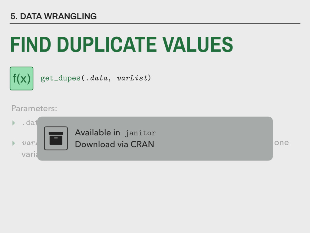
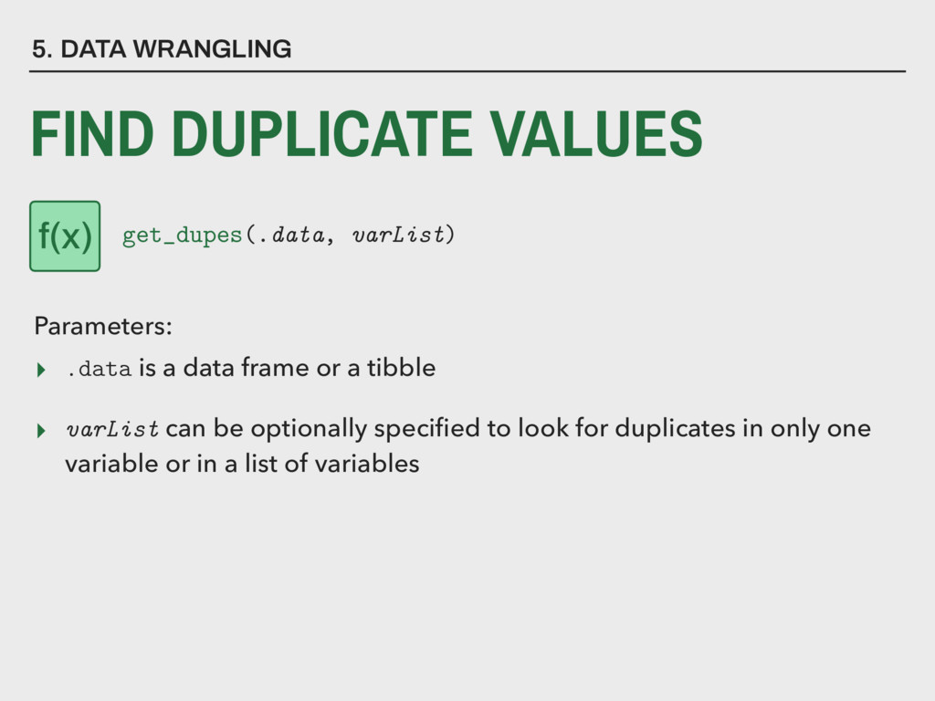
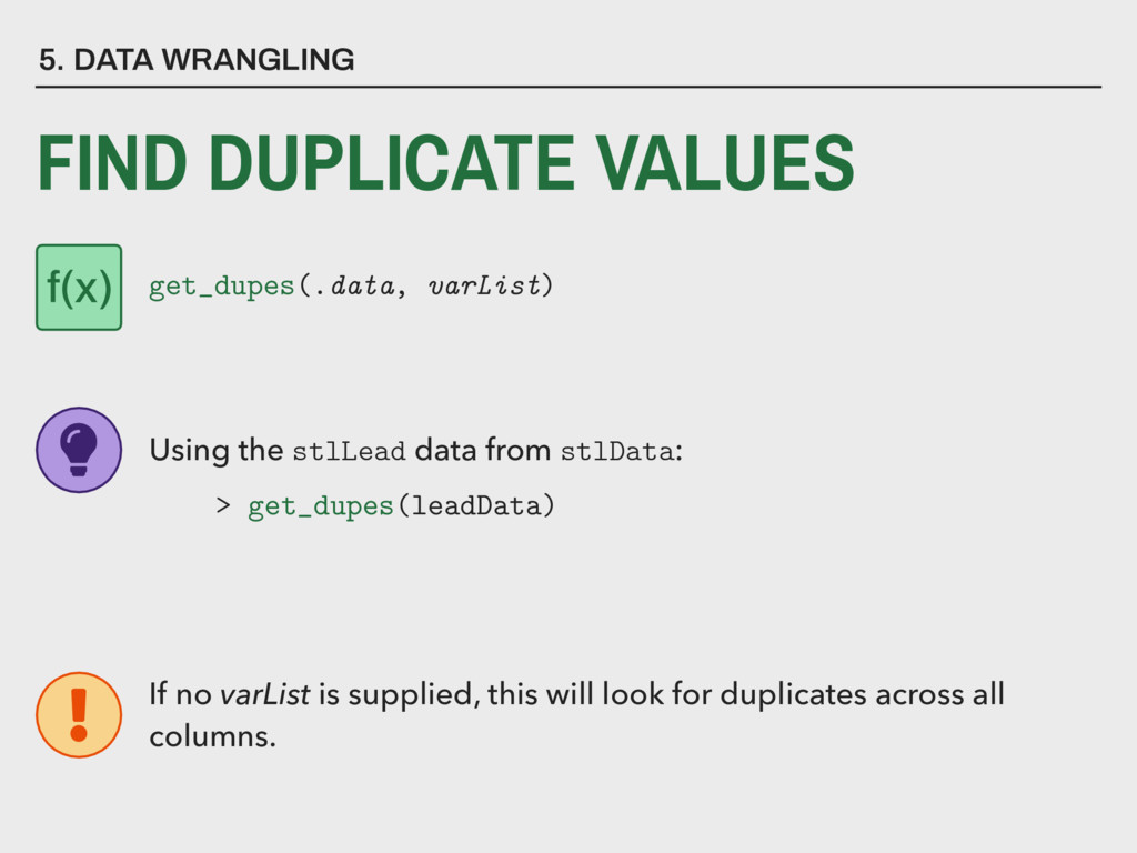
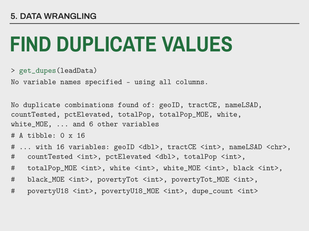
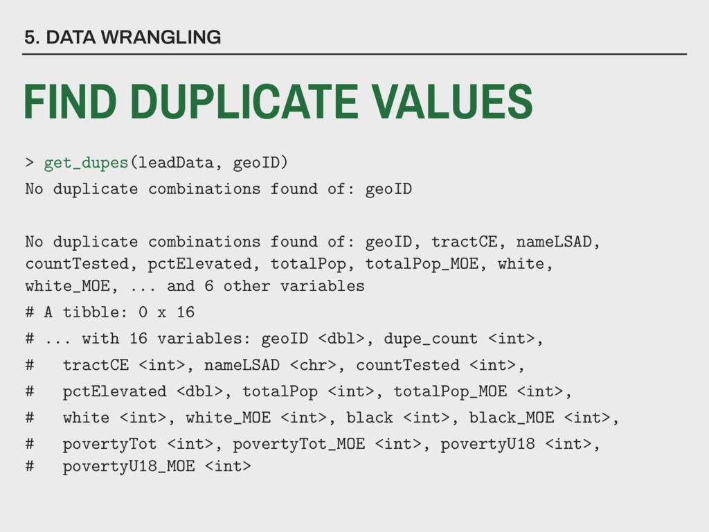
88. ▸ .data is a data frame or a tibble ▸ varList can be optionally specified to look for duplicates in only one variable or in a list of variables Available in janitor
 Download via CRAN 5. DATA WRANGLING FIND DUPLICATE VALUES Parameters: get_dupes(.data, varList) f(x)
89. ▸ .data is a data frame or a tibble ▸ varList can be optionally specified to look for duplicates in only one variable or in a list of variables 5. DATA WRANGLING FIND DUPLICATE VALUES Parameters: get_dupes(.data, varList) f(x)
90. f(x) 5. DATA WRANGLING FIND DUPLICATE VALUES get_dupes(.data, varList) Using the stlLead data from stlData: > get_dupes(leadData) If no varList is supplied, this will look for duplicates across all columns.
91. 5. DATA WRANGLING FIND DUPLICATE VALUES > get_dupes(leadData) No variable names specified - using all columns. No duplicate combinations found of: geoID, tractCE, nameLSAD, countTested, pctElevated, totalPop, totalPop_MOE, white, white_MOE, ... and 6 other variables # A tibble: 0 x 16 # ... with 16 variables: geoID <dbl>, tractCE <int>, nameLSAD <chr>, # countTested <int>, pctElevated <dbl>, totalPop <int>, # totalPop_MOE <int>, white <int>, white_MOE <int>, black <int>, # black_MOE <int>, povertyTot <int>, povertyTot_MOE <int>, # povertyU18 <int>, povertyU18_MOE <int>, dupe_count <int>
92. 5. DATA WRANGLING FIND DUPLICATE VALUES > get_dupes(leadData, geoID) No duplicate combinations found of: geoID No duplicate combinations found of: geoID, tractCE, nameLSAD, countTested, pctElevated, totalPop, totalPop_MOE, white, white_MOE, ... and 6 other variables # A tibble: 0 x 16 # ... with 16 variables: geoID <dbl>, dupe_count <int>, # tractCE <int>, nameLSAD <chr>, countTested <int>, # pctElevated <dbl>, totalPop <int>, totalPop_MOE <int>, # white <int>, white_MOE <int>, black <int>, black_MOE <int>, # povertyTot <int>, povertyTot_MOE <int>, povertyU18 <int>, 
 # povertyU18_MOE <int>
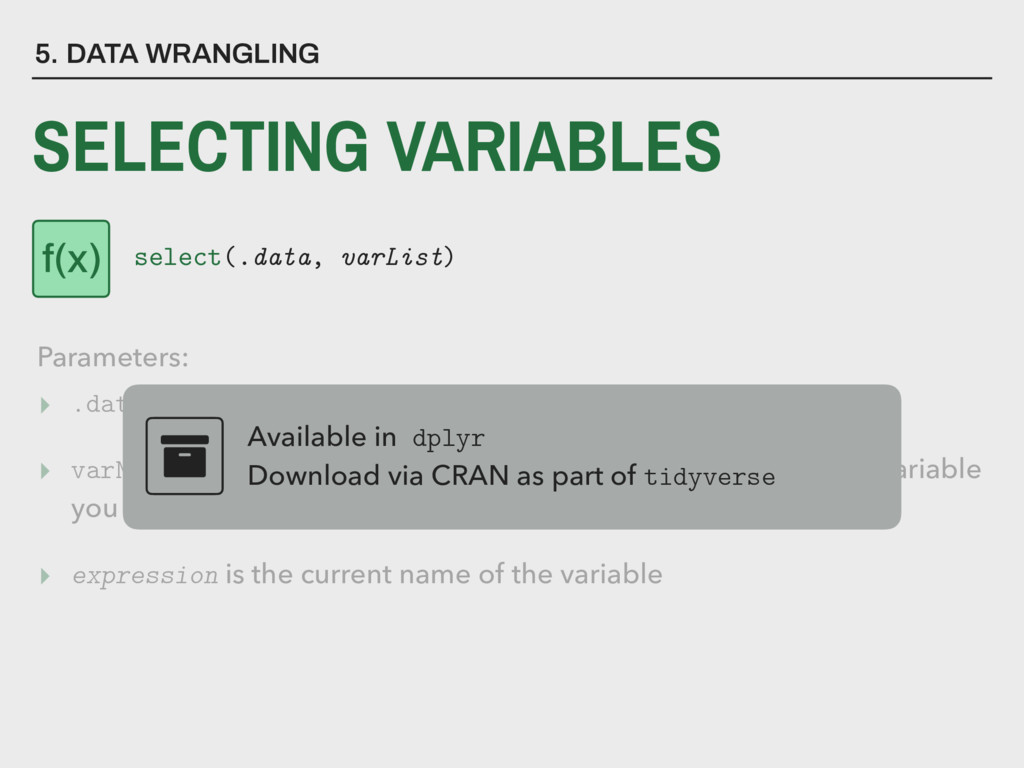
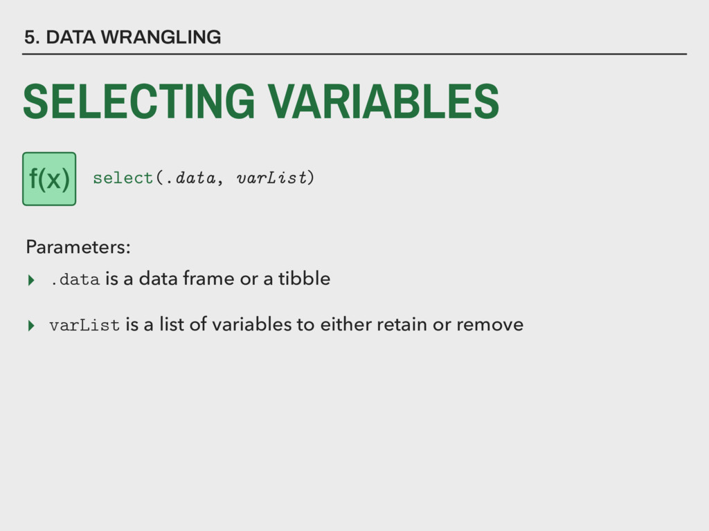
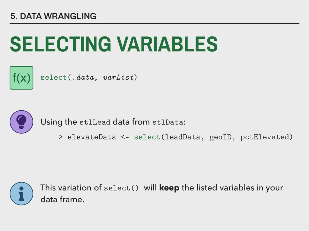
93. ▸ .data is a data frame or a tibble ▸ varName is either an existing variable you want to edit or a new variable you want to create ▸ expression is the current name of the variable Available in dplyr
 Download via CRAN as part of tidyverse 5. DATA WRANGLING SELECTING VARIABLES Parameters: select(.data, varList) f(x)
94. ▸ .data is a data frame or a tibble ▸ varList is a list of variables to either retain or remove 5. DATA WRANGLING SELECTING VARIABLES Parameters: select(.data, varList) f(x)
95. f(x) 5. DATA WRANGLING SELECTING VARIABLES select(.data, varList) Using the stlLead data from stlData: > elevateData <- select(leadData, geoID, pctElevated) This variation of select() will keep the listed variables in your data frame.
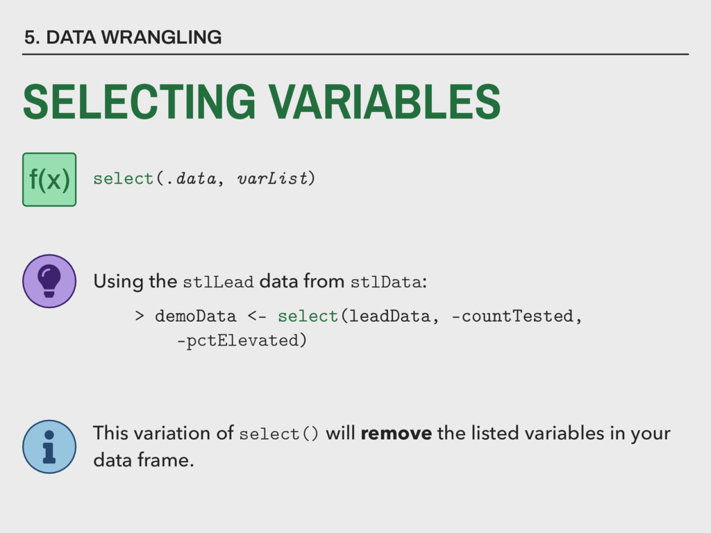
96. f(x) 5. DATA WRANGLING SELECTING VARIABLES select(.data, varList) Using the stlLead data from stlData: > demoData <- select(leadData, -countTested, 
 —pctElevated) This variation of select() will remove the listed variables in your data frame.
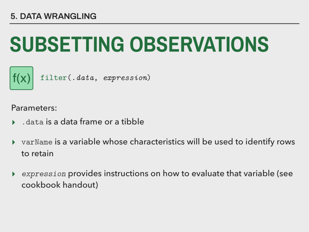
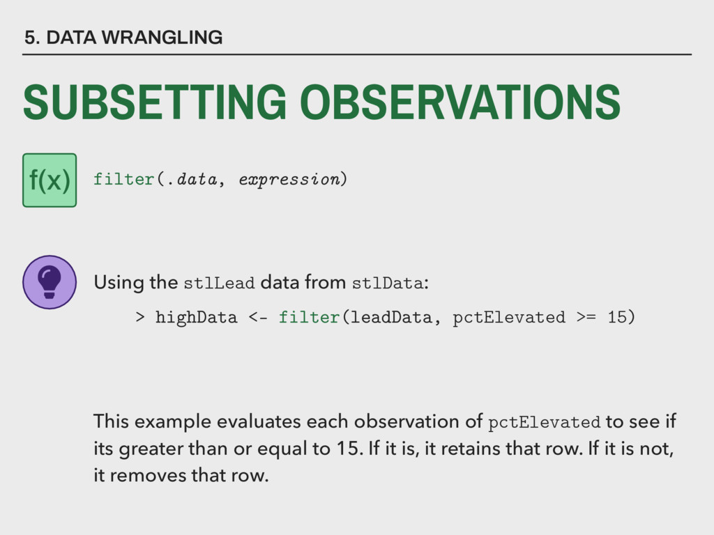
97. ▸ .data is a data frame or a tibble ▸ varName is a variable whose characteristics will be used to identify rows to retain ▸ expression provides instructions on how to evaluate that variable (see cookbook handout) 5. DATA WRANGLING SUBSETTING OBSERVATIONS Parameters: filter(.data, expression) f(x)
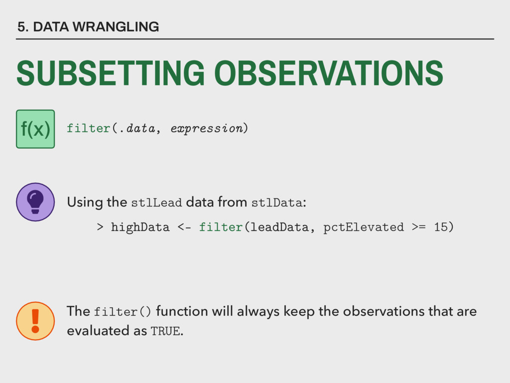
98. f(x) 5. DATA WRANGLING SUBSETTING OBSERVATIONS filter(.data, expression) Using the stlLead data from stlData: > highData <- filter(leadData, pctElevated >= 15) The filter() function will always keep the observations that are evaluated as TRUE.
99. f(x) 5. DATA WRANGLING SUBSETTING OBSERVATIONS filter(.data, expression) Using the stlLead data from stlData: > highData <- filter(leadData, pctElevated >= 15) This example evaluates each observation of pctElevated to see if its greater than or equal to 15. If it is, it retains that row. If it is not, it removes that row.
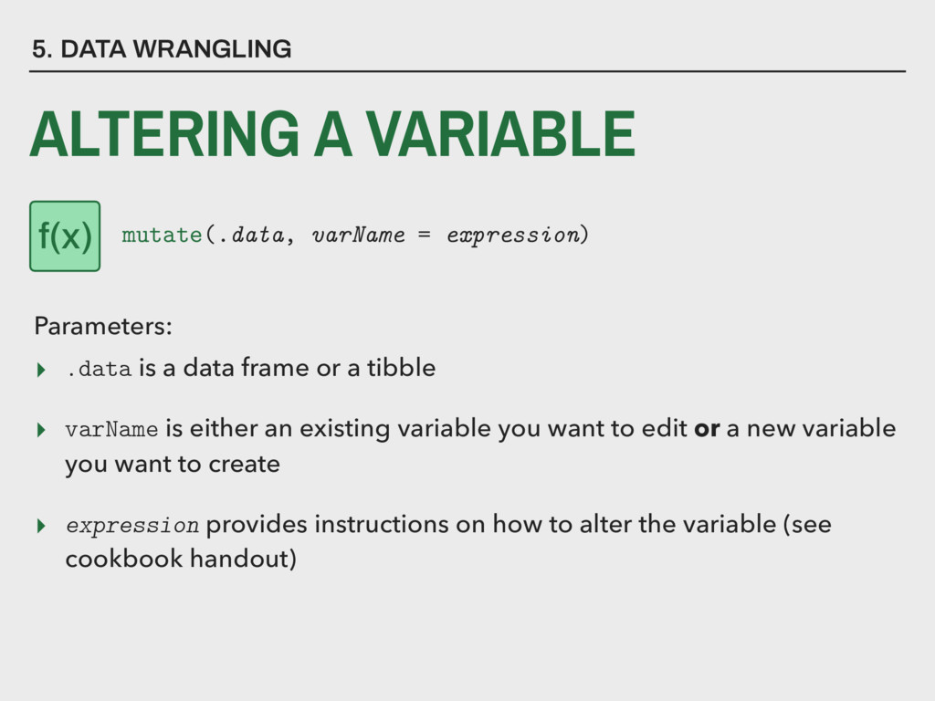
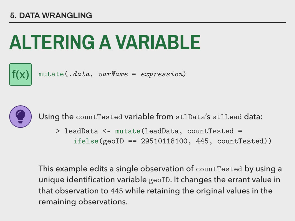
100. ▸ .data is a data frame or a tibble ▸ varName is either an existing variable you want to edit or a new variable you want to create ▸ expression provides instructions on how to alter the variable (see cookbook handout) 5. DATA WRANGLING ALTERING A VARIABLE Parameters: mutate(.data, varName = expression) f(x)
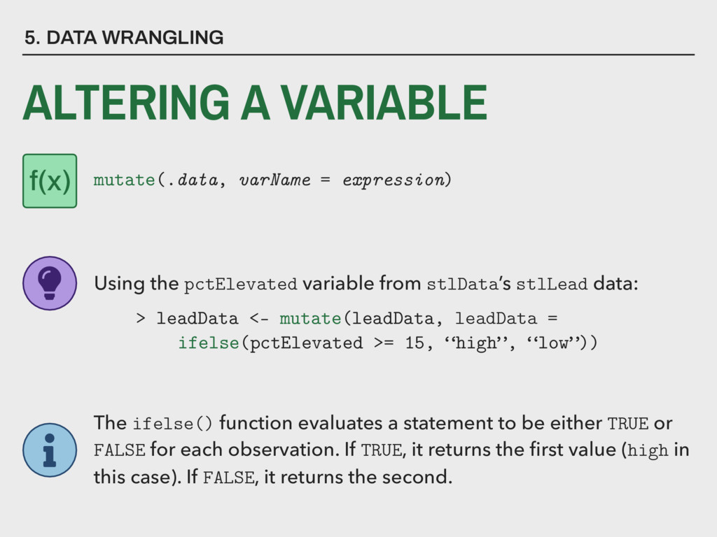
101. f(x) 5. DATA WRANGLING ALTERING A VARIABLE mutate(.data, varName = expression) Using the pctElevated variable from stlData’s stlLead data: > leadData <- mutate(leadData, leadData = 
 ifelse(pctElevated >= 15, “high”, “low”)) The ifelse() function evaluates a statement to be either TRUE or FALSE for each observation. If TRUE, it returns the first value (high in this case). If FALSE, it returns the second.
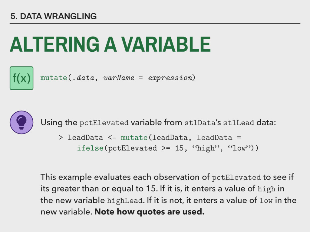
102. f(x) 5. DATA WRANGLING ALTERING A VARIABLE mutate(.data, varName = expression) Using the pctElevated variable from stlData’s stlLead data: > leadData <- mutate(leadData, leadData = 
 ifelse(pctElevated >= 15, “high”, “low”)) This example evaluates each observation of pctElevated to see if its greater than or equal to 15. If it is, it enters a value of high in the new variable highLead. If it is not, it enters a value of low in the new variable. Note how quotes are used.
103. f(x) 5. DATA WRANGLING ALTERING A VARIABLE mutate(.data, varName = expression) Using the countTested variable from stlData’s stlLead data: > leadData <- mutate(leadData, countTested = 
 ifelse(geoID == 29510118100, 445, countTested)) This example edits a single observation of countTested by using a unique identification variable geoID. It changes the errant value in that observation to 445 while retaining the original values in the remaining observations.
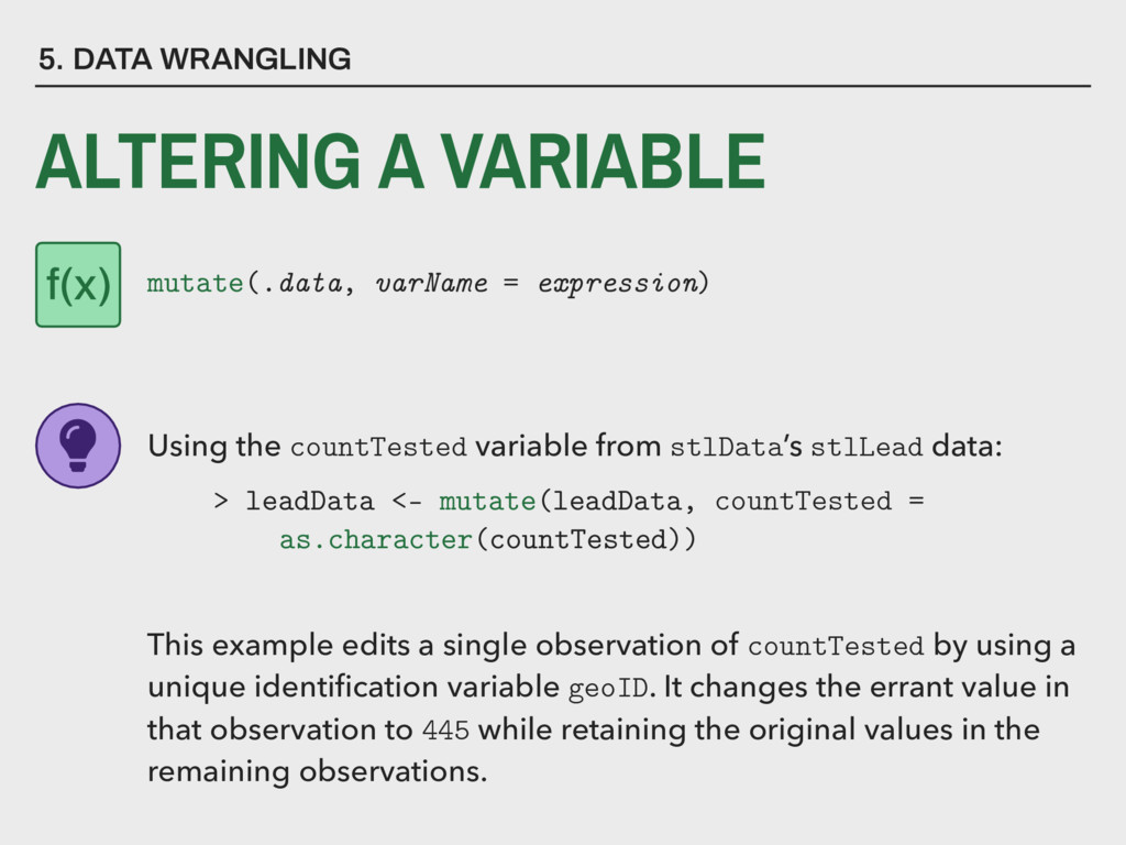
104. f(x) 5. DATA WRANGLING ALTERING A VARIABLE mutate(.data, varName = expression) Using the countTested variable from stlData’s stlLead data: > leadData <- mutate(leadData, countTested = 
 as.character(countTested)) This example edits a single observation of countTested by using a unique identification variable geoID. It changes the errant value in that observation to 445 while retaining the original values in the remaining observations.
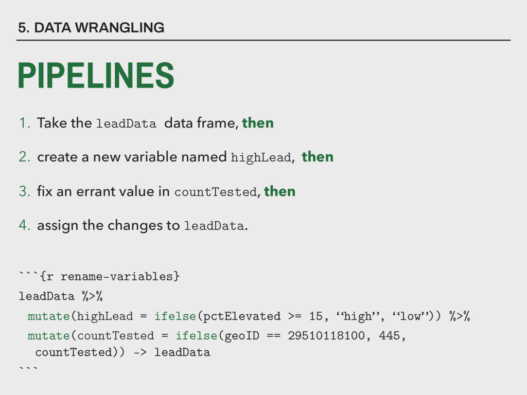
105. 5. DATA WRANGLING PIPELINES ```{r rename-variables} leadData %>% mutate(highLead = ifelse(pctElevated >= 15, “high”, “low”)) %>% mutate(countTested = ifelse(geoID == 29510118100, 445, 
 countTested)) -> leadData ``` 1. Take the leadData data frame, then 2. create a new variable named highLead, then 3. fix an errant value in countTested, then 4. assign the changes to leadData.
106. 6 BACK 
 MATTER
107. AGENDA REVIEW 6. BACK MATTER 2. GISc & Public Policy 3. Types of Data 4. Methodological Challenges in GISc 5. Data Wrangling
108. REMINDERS #. BACK MATTER LP-04, Lab-02, and PS-01 are all due next class (February 12th) We’ll be putting final project workgroups together this week. Please close any open GitHub Issues in your assignment repository!