SOC 4930 & SOC 5050 - Week 11

Lecture slides for Week 10 of the Saint Louis University Course Quantitative Analysis: Applied Inferential Statistics. These slides cover the topics related to correlation analyses.

Transcript

1. CORRELATION 
 (PART 2) QUANTITATIVE ANALYSIS CHRISTOPHER PRENER, PH.D. FALL 2018 WEEK 11 LECTURE 11
2. AGENDA QUANTITATIVE ANALYSIS / WEEK 11 / LECTURE 11 1. Front Matter 2. More with knitr 3. Scatterplots 4. Matrix Arrays 5. Correlation in R 6. Power Analyses for Correlation 7. Back Matter
3. 1 FRONT 
 MATTER
4. 1. FRONT MATTER ANNOUNCEMENTS ITS or DPS issues? Lab 10 and Problem Set 05 due next Monday as is peer review of partner’s materials! Draft papers due next Monday! Reminder - no additional lecture preps!
5. MORE WITH KNITR 2
6. IN-LINE CODE ```{r load-data} library(ggplot2) auto <- mpg ``` The average highway fuel efficiency in the data set is `r mean(auto$hwy)`. 2. MORE WITH KNITR
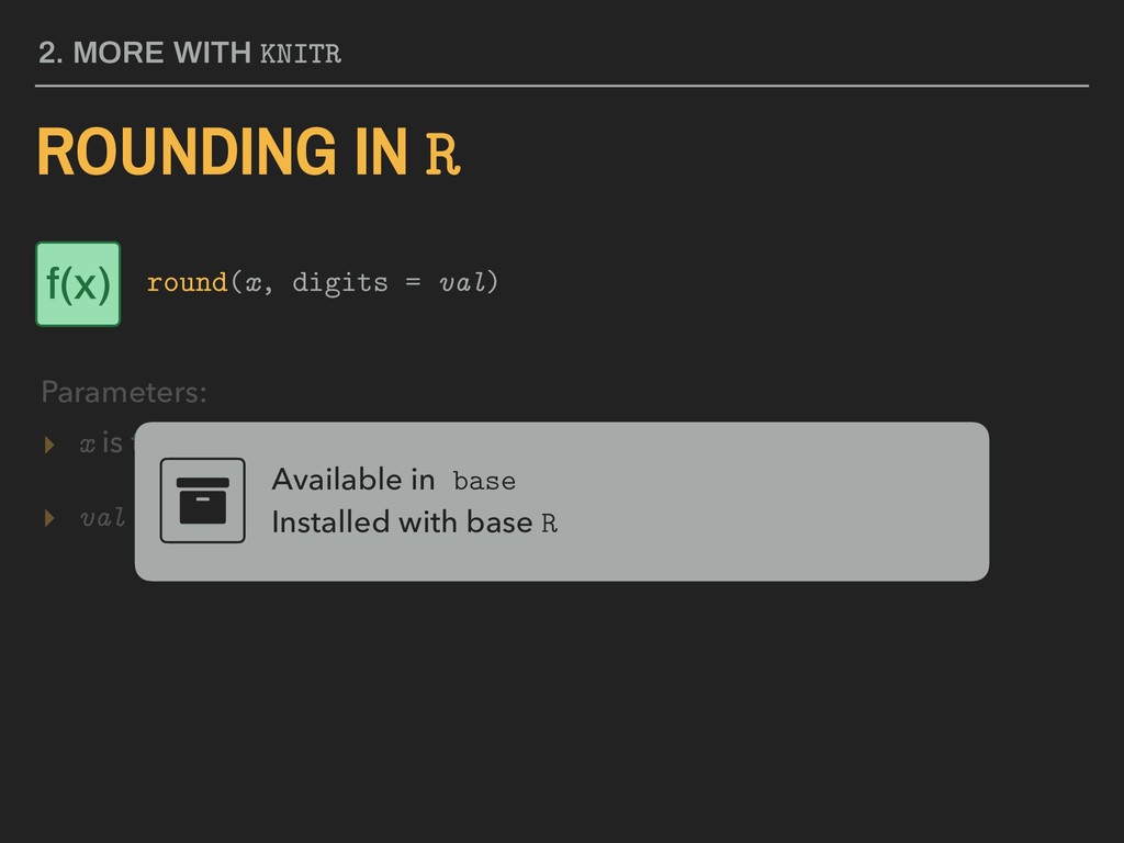
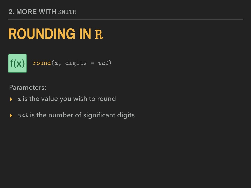
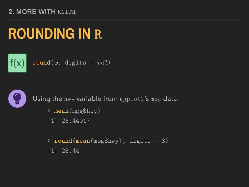
7. ▸ x is the value you wish to round ▸ val is the number of significant digitsval Available in base
 Installed with base R 2. MORE WITH KNITR ROUNDING IN R Parameters: round(x, digits = val) f(x)
8. ▸ x is the value you wish to round ▸ val is the number of significant digits 2. MORE WITH KNITR ROUNDING IN R Parameters: round(x, digits = val) f(x)
9. ROUNDING IN R 2. MORE WITH KNITR round(x, digits = val) Using the hwy variable from ggplot2’s mpg data: > mean(mpg$hwy) [1] 23.44017 > round(mean(mpg$hwy), digits = 3) [1] 23.44 f(x)
10. ROUNDED IN-LINE CODE ```{r load-data} library(ggplot2) auto <- mpg ``` The average highway fuel efficiency in the data set is `r round(mean(auto$hwy), digits = 3)`. 2. MORE WITH KNITR
11. \x{} 2. MORE WITH KNITR “IT’S ALL GREEK TO ME” $ \mu \sigma {\sigma}^{2} $
12. 2. MORE WITH KNITR MATHEMATICAL OPERATORS $ r = \sqrt{{r}^{2}} $ \x{} r = r2
13. 2. MORE WITH KNITR MATHEMATICAL SYMBOLS $ {(x-\bar{x})}^{2} $ \x{} (x − ¯ x)2
14. 2. MORE WITH KNITR PEARSON’S R
15. \x{} 2. MORE WITH KNITR PEARSON’S R r = Pn i=1 (x ¯ x)(y ¯ y) (n 1)sxsy \sum_{i=1}^{n}
16. 2. MORE WITH KNITR PEARSON’S R r = Pn i=1 (x ¯ x)(y ¯ y) (n 1)sxsy \bar{x} \x{}
17. 2. MORE WITH KNITR PEARSON’S R r = Pn i=1 (x ¯ x)(y ¯ y) (n 1)sxsy \sum_{i=1}^{n}{(x-\bar{x})(y-\bar{y})} \x{}
18. 2. MORE WITH KNITR PEARSON’S R r = Pn i=1 (x ¯ x)(y ¯ y) (n 1)sxsy {s}_{x} \x{}
19. 2. MORE WITH KNITR PEARSON’S R r = Pn i=1 (x ¯ x)(y ¯ y) (n 1)sxsy (n-1){s}_{x}{s}_{y} \x{}
20. 2. MORE WITH KNITR PEARSON’S R r = Pn i=1 (x ¯ x)(y ¯ y) (n 1)sxsy \frac{}{} \x{}
21. 2. MORE WITH KNITR PEARSON’S R $ r = \frac{\sum_{i=1}^{n}{(x-\bar{x})(y-\bar{y})}}
 {(n-1){s}_{x}{s}_{y}} $ \x{}
22. SCATTERPLOTS 3
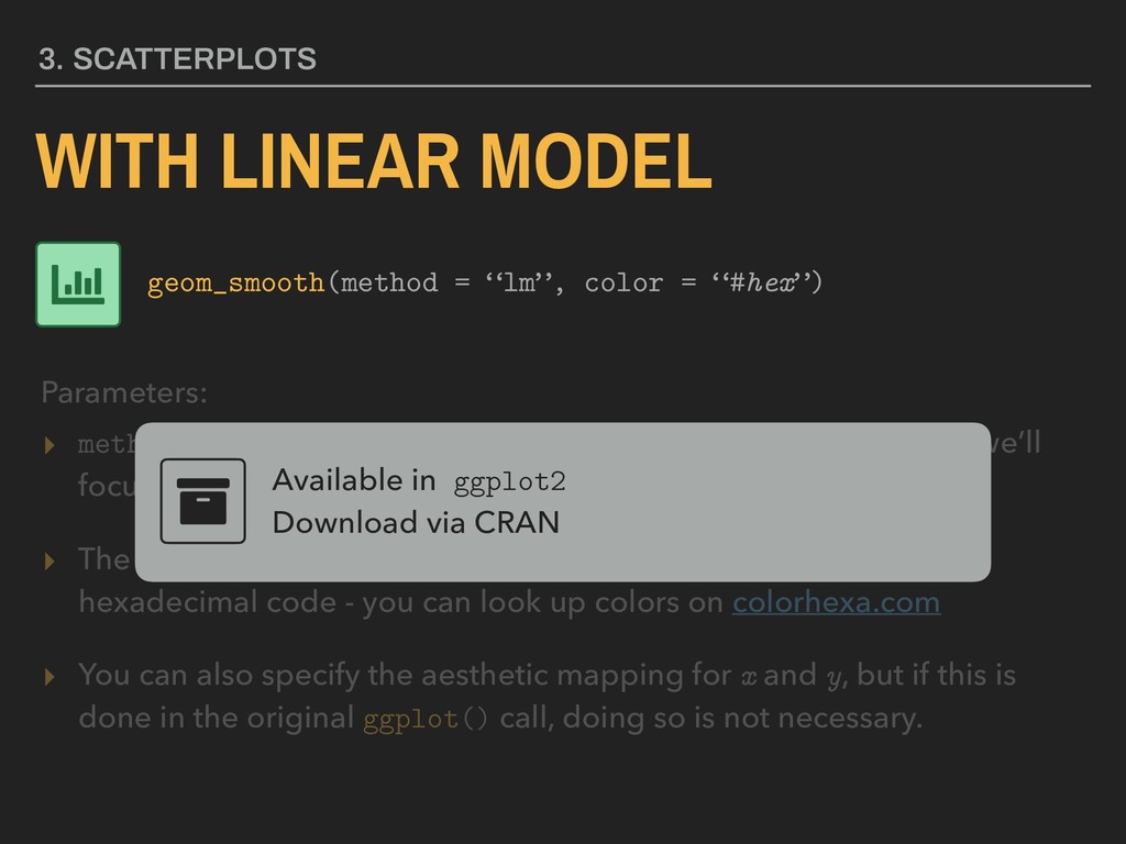
23. ▸ method is the parameter that specifies the type of model to use; we’ll focus on using linear models (“lm”) this semester ▸ The hex value will assign a color to the line using a six digit hexadecimal code - you can look up colors on colorhexa.com ▸ You can also specify the aesthetic mapping for x and y, but if this is done in the original ggplot() call, doing so is not necessary. Available in ggplot2
 Download via CRAN 3. SCATTERPLOTS WITH LINEAR MODEL Parameters: geom_smooth(method = “lm”, color = “#hex”)
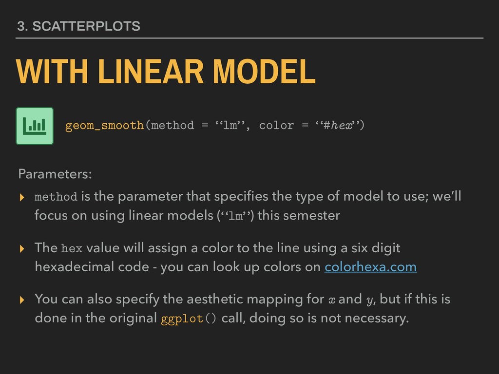
24. ▸ method is the parameter that specifies the type of model to use; we’ll focus on using linear models (“lm”) this semester ▸ The hex value will assign a color to the line using a six digit hexadecimal code - you can look up colors on colorhexa.com ▸ You can also specify the aesthetic mapping for x and y, but if this is done in the original ggplot() call, doing so is not necessary. 3. SCATTERPLOTS WITH LINEAR MODEL Parameters: geom_smooth(method = “lm”, color = “#hex”)
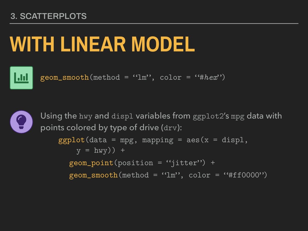
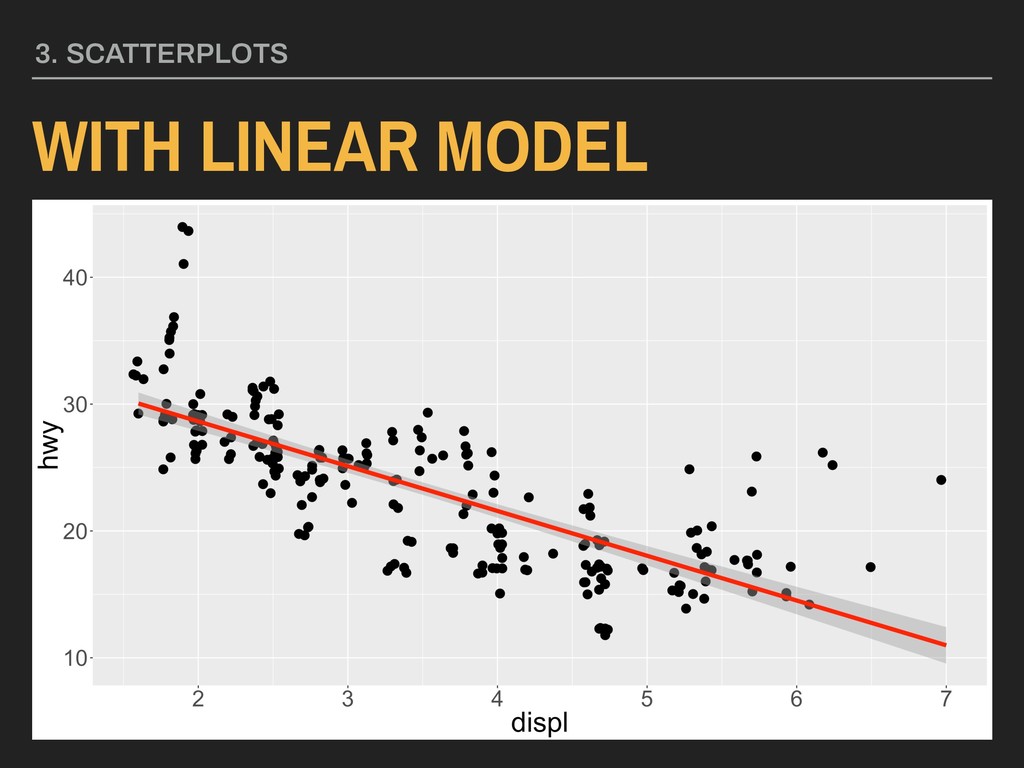
25. WITH LINEAR MODEL 3. SCATTERPLOTS geom_smooth(method = “lm”, color = “#hex”) Using the hwy and displ variables from ggplot2’s mpg data with points colored by type of drive (drv): ggplot(data = mpg, mapping = aes(x = displ, 
 y = hwy)) + geom_point(position = “jitter”) + geom_smooth(method = “lm”, color = “#ff0000”)
26. WITH LINEAR MODEL 3. SCATTERPLOTS
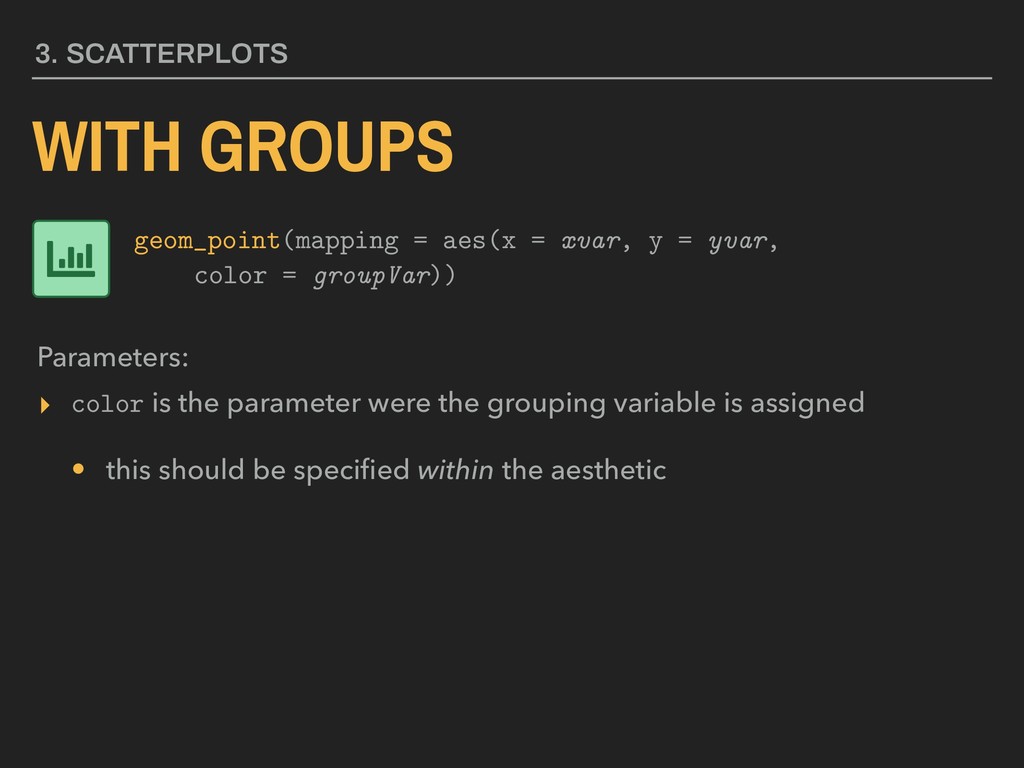
27. ▸ color is the parameter were the grouping variable is assigned • this should be specified within the aesthetic 3. SCATTERPLOTS WITH GROUPS Parameters: geom_point(mapping = aes(x = xvar, y = yvar, 
 color = groupVar))
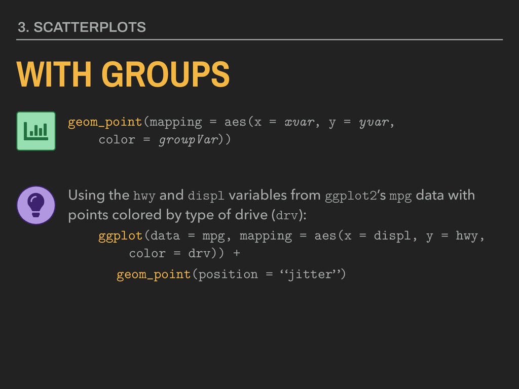
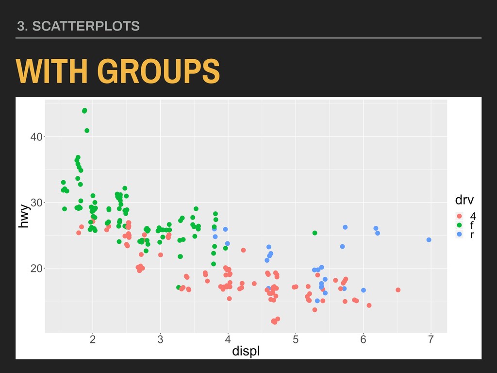
28. WITH GROUPS 3. SCATTERPLOTS geom_point(mapping = aes(x = xvar, y = yvar, 
 color = groupVar)) Using the hwy and displ variables from ggplot2’s mpg data with points colored by type of drive (drv): ggplot(data = mpg, mapping = aes(x = displ, y = hwy, 
 color = drv)) + geom_point(position = “jitter”)
29. WITH GROUPS 3. SCATTERPLOTS
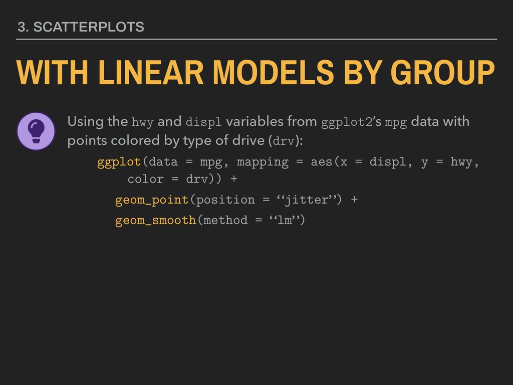
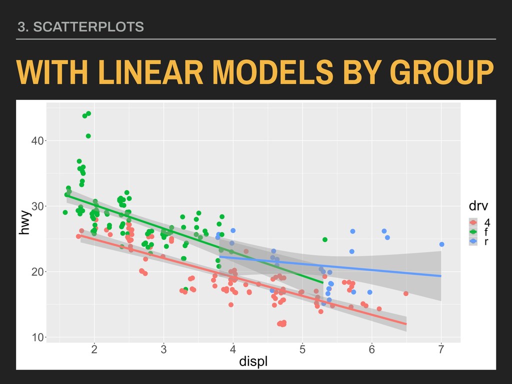
30. Using the hwy and displ variables from ggplot2’s mpg data with points colored by type of drive (drv): WITH LINEAR MODELS BY GROUP 3. SCATTERPLOTS ggplot(data = mpg, mapping = aes(x = displ, y = hwy, 
 color = drv)) + geom_point(position = “jitter”) + geom_smooth(method = “lm”)
31. WITH LINEAR MODELS BY GROUP 3. SCATTERPLOTS
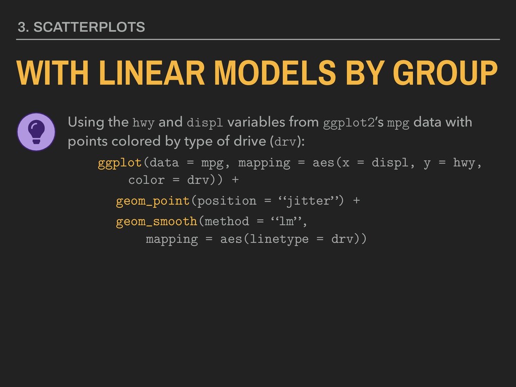
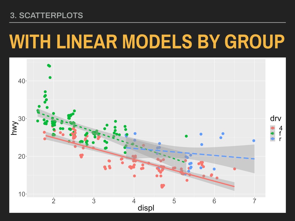
32. Using the hwy and displ variables from ggplot2’s mpg data with points colored by type of drive (drv): WITH LINEAR MODELS BY GROUP 3. SCATTERPLOTS ggplot(data = mpg, mapping = aes(x = displ, y = hwy, 
 color = drv)) + geom_point(position = “jitter”) + geom_smooth(method = “lm”, 
 mapping = aes(linetype = drv))
33. WITH LINEAR MODELS BY GROUP 3. SCATTERPLOTS
34. ▸ facetVar is the parameter were the faceting variable is assigned 3. SCATTERPLOTS WITH FACETS Parameters: facet_grid(. ~ facetVar)
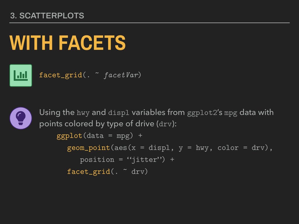
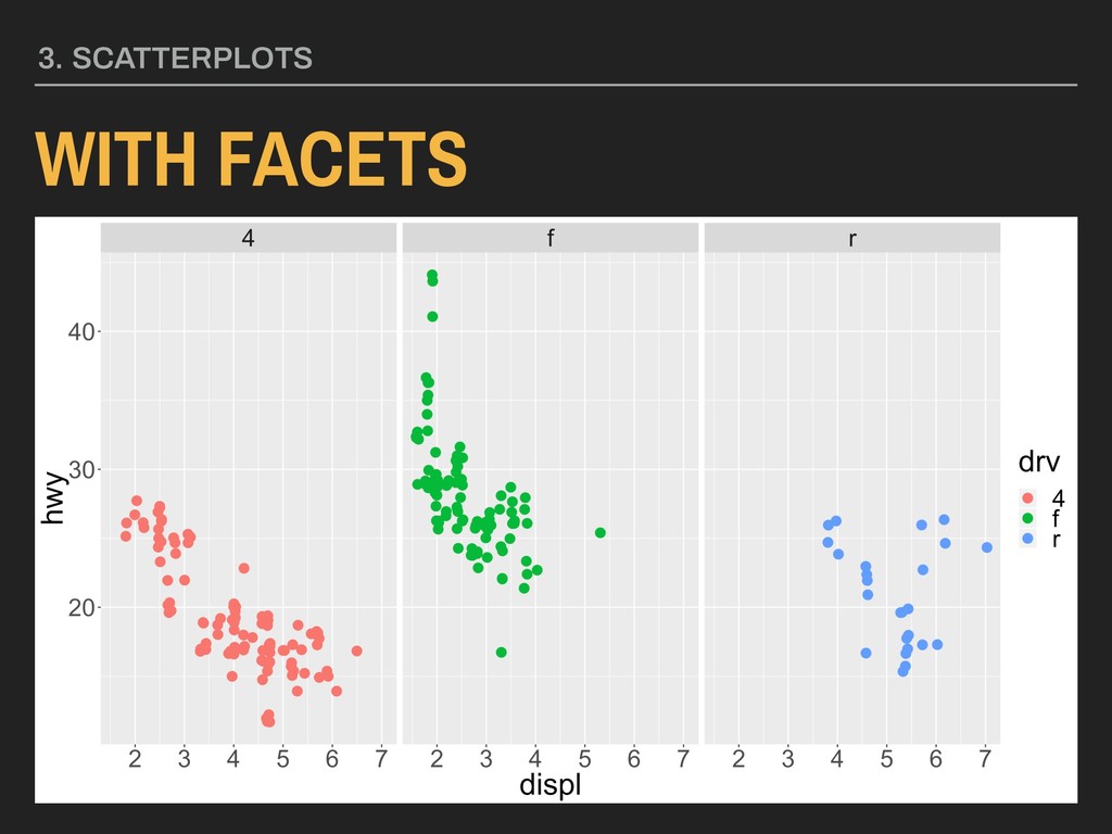
35. WITH FACETS 3. SCATTERPLOTS facet_grid(. ~ facetVar) Using the hwy and displ variables from ggplot2’s mpg data with points colored by type of drive (drv): ggplot(data = mpg) + geom_point(aes(x = displ, y = hwy, color = drv), position = “jitter”) + facet_grid(. ~ drv)
36. WITH FACETS 3. SCATTERPLOTS
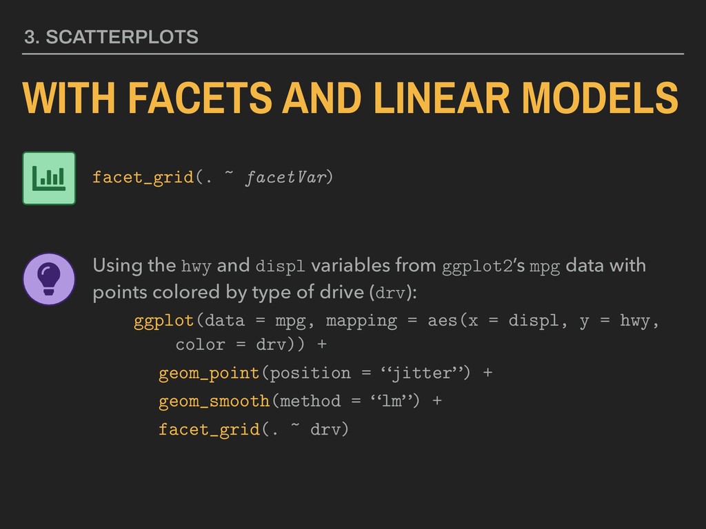
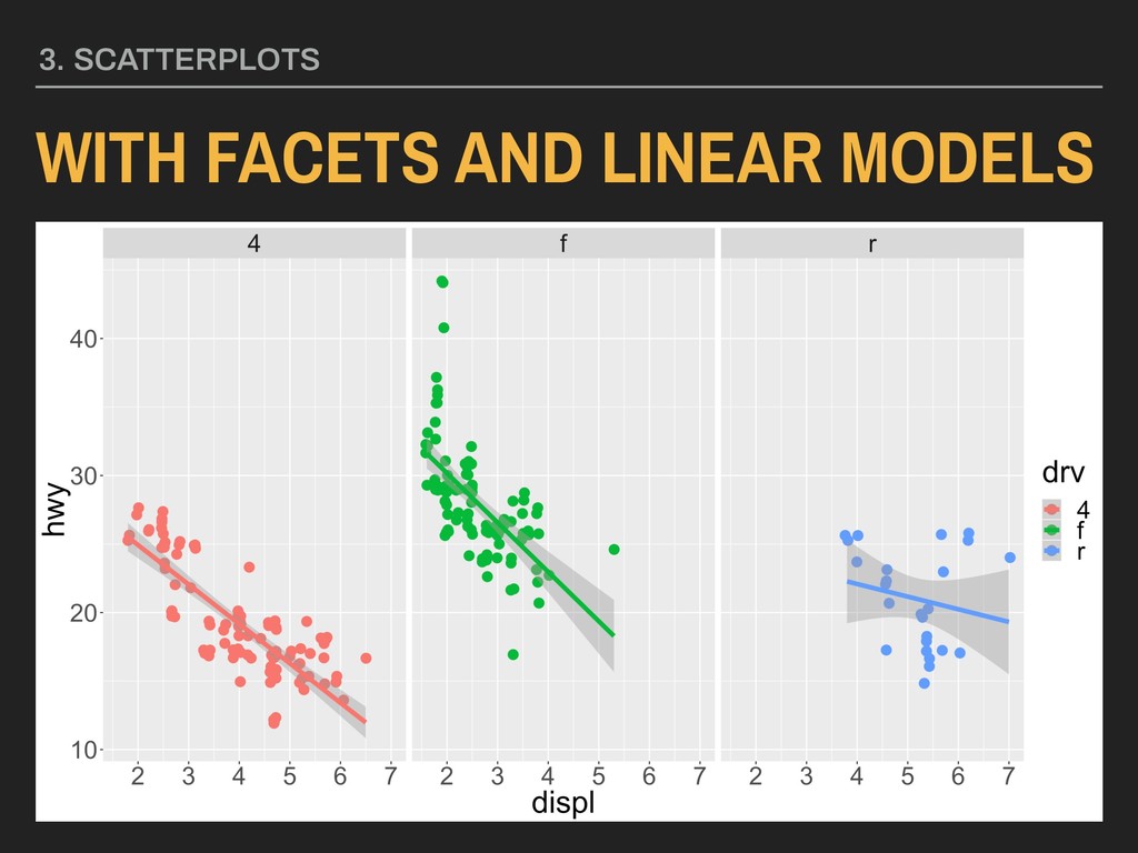
37. WITH FACETS AND LINEAR MODELS 3. SCATTERPLOTS facet_grid(. ~ facetVar) Using the hwy and displ variables from ggplot2’s mpg data with points colored by type of drive (drv): ggplot(data = mpg, mapping = aes(x = displ, y = hwy, color = drv)) + geom_point(position = “jitter”) + geom_smooth(method = “lm”) + facet_grid(. ~ drv)
38. WITH FACETS AND LINEAR MODELS 3. SCATTERPLOTS
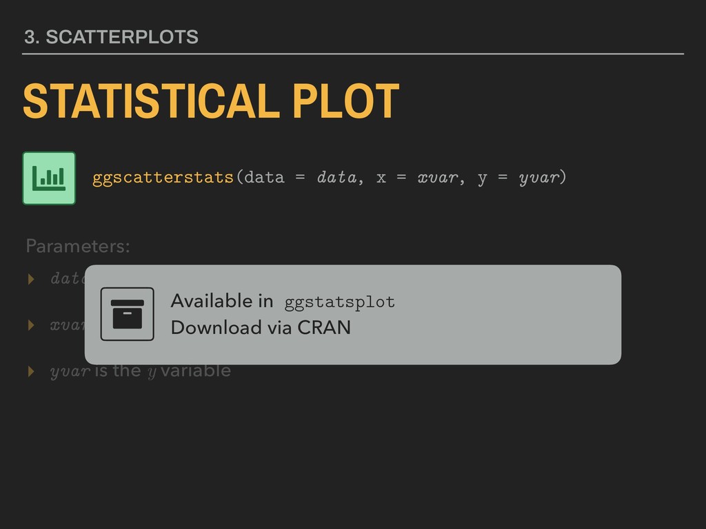
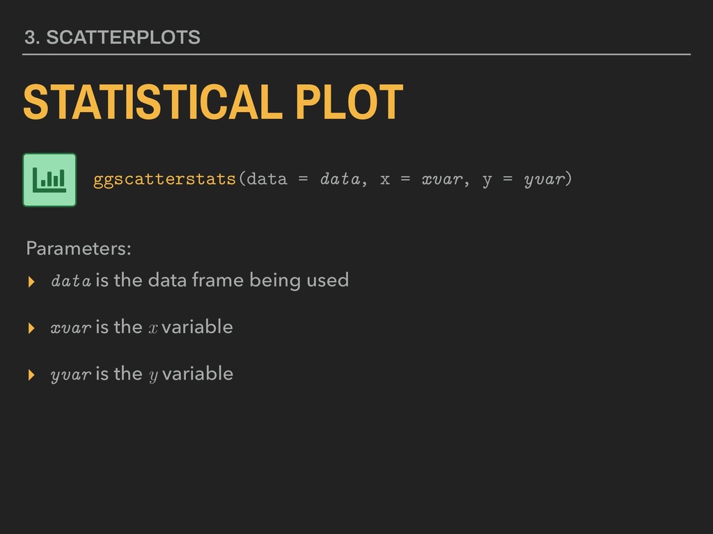
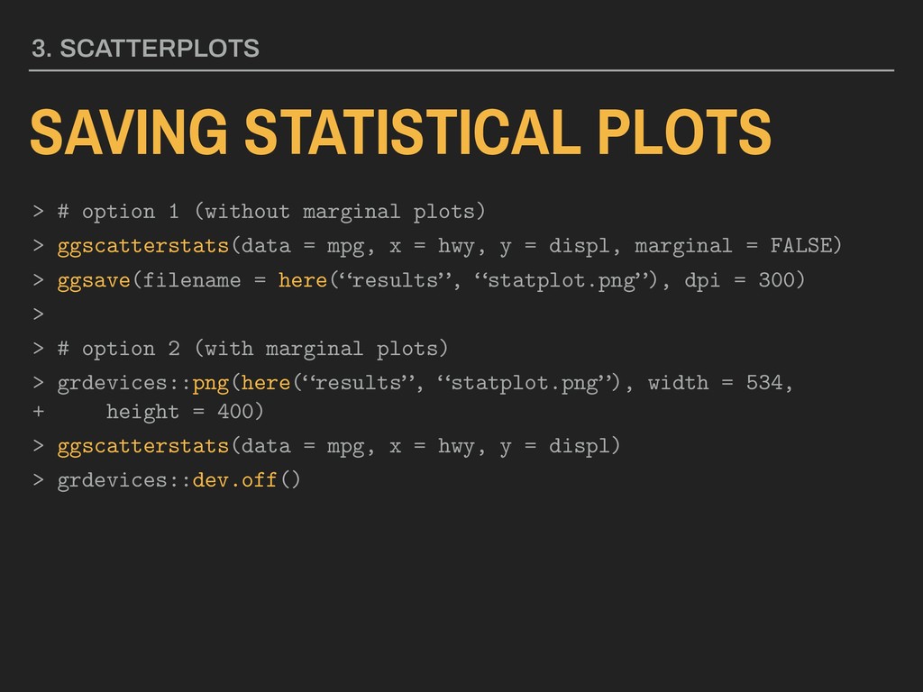
39. ▸ data is the data frame being used ▸ xvar is the x variable ▸ yvar is the y variable Available in ggstatsplot
 Download via CRAN 3. SCATTERPLOTS STATISTICAL PLOT Parameters: ggscatterstats(data = data, x = xvar, y = yvar)
40. ▸ data is the data frame being used ▸ xvar is the x variable ▸ yvar is the y variable 3. SCATTERPLOTS STATISTICAL PLOT Parameters: ggscatterstats(data = data, x = xvar, y = yvar)
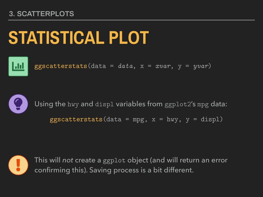
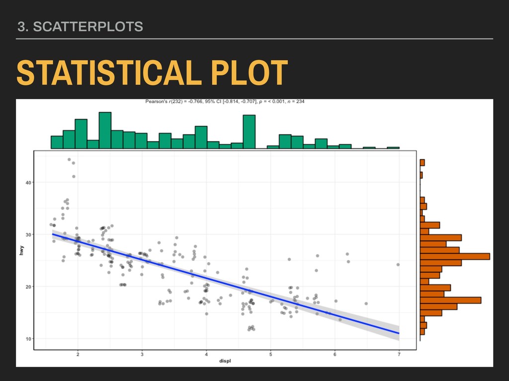
41. STATISTICAL PLOT 3. SCATTERPLOTS ggscatterstats(data = data, x = xvar, y = yvar) Using the hwy and displ variables from ggplot2’s mpg data: ggscatterstats(data = mpg, x = hwy, y = displ) This will not create a ggplot object (and will return an error confirming this). Saving process is a bit different.
42. STATISTICAL PLOT 3. SCATTERPLOTS
43. SAVING STATISTICAL PLOTS > # option 1 (without marginal plots) > ggscatterstats(data = mpg, x = hwy, y = displ, marginal = FALSE) > ggsave(filename = here(“results”, “statplot.png”), dpi = 300) > > # option 2 (with marginal plots) > grdevices::png(here(“results”, “statplot.png”), width = 534, 
 + height = 400) > ggscatterstats(data = mpg, x = hwy, y = displ) > grdevices::dev.off() 3. SCATTERPLOTS
44. MATRIX ARRAYS 4
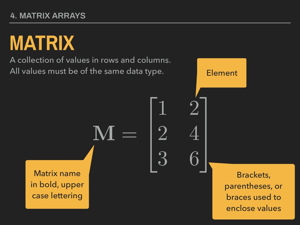
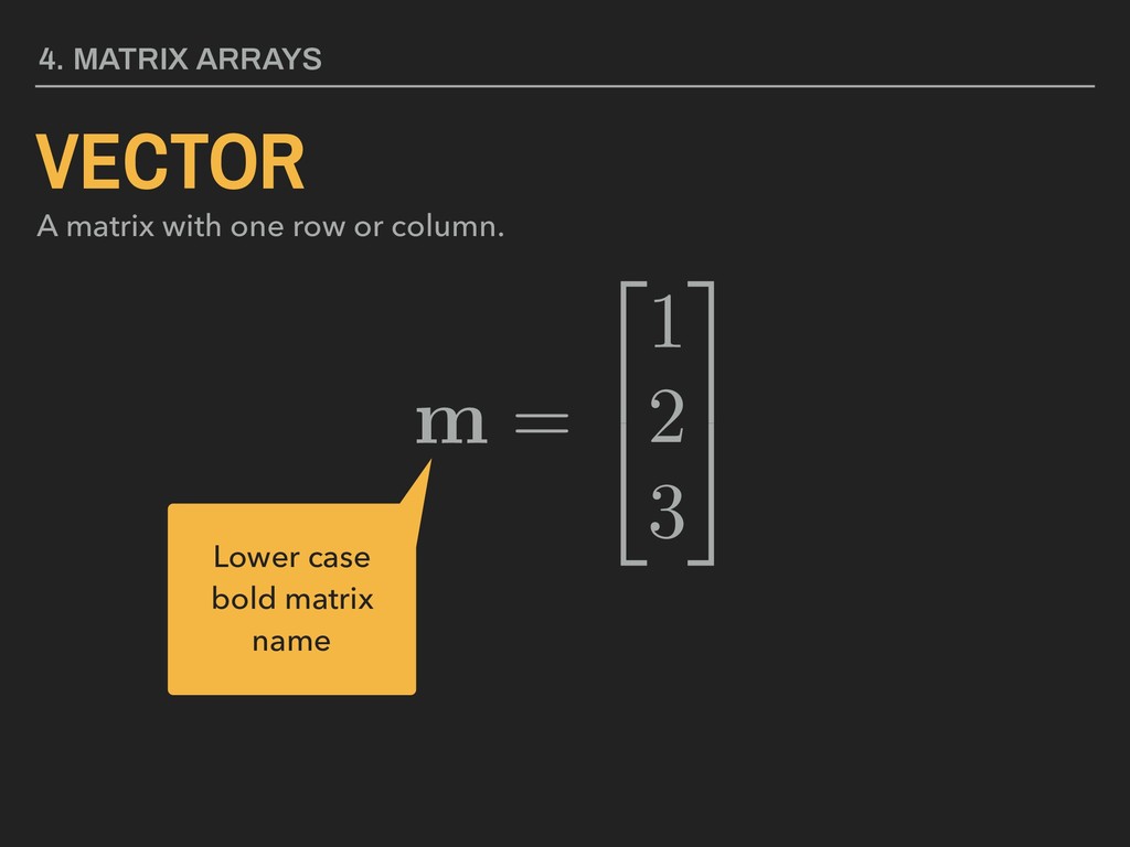
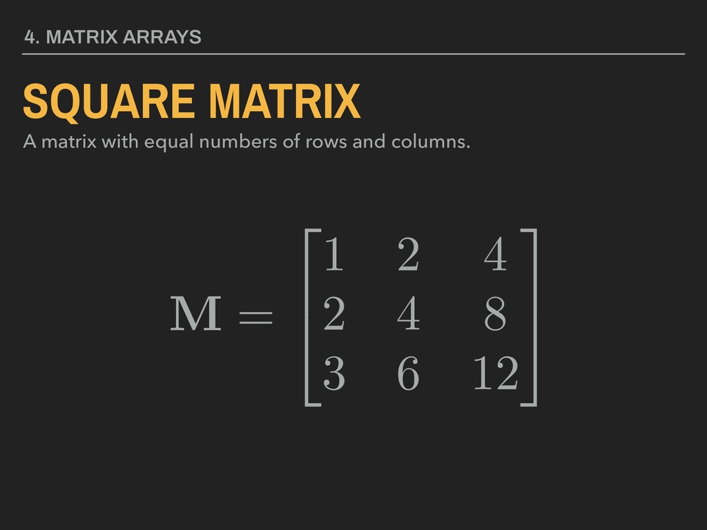
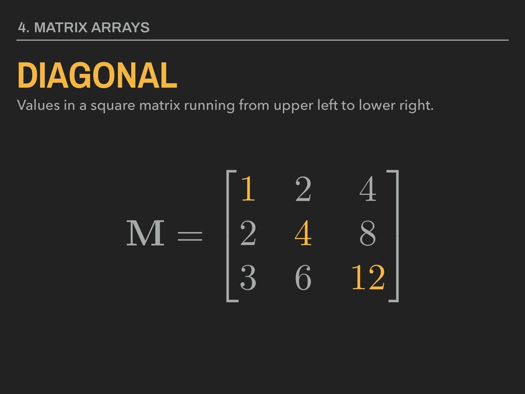
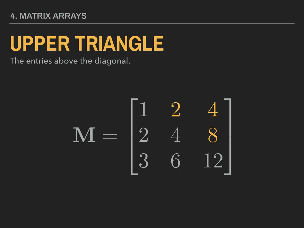
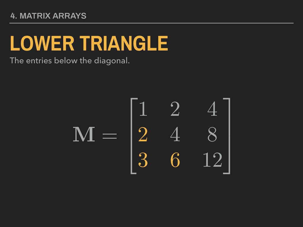
45. M = 2 4 1 2 2 4 3 6 3 5 4. MATRIX ARRAYS MATRIX A collection of values in rows and columns. 
 All values must be of the same data type. Matrix name in bold, upper case lettering Brackets, parentheses, or braces used to enclose values Element
46. 4. MATRIX ARRAYS SCALAR A matrix with one element. m = ⇥ 1 ⇤ Lower case italicized matrix name
47. 4. MATRIX ARRAYS SCALAR All single values saved to an object in R are scalars. > m <- 1 > m1 <- TRUE > m2 <- “ham”
48. 4. MATRIX ARRAYS VECTOR A matrix with one row or column. m = 2 4 1 2 3 3 5 Lower case bold matrix name
49. 4. MATRIX ARRAYS ATOMIC VECTOR R’s simplest data type. m = 2 4 1 2 3 3 5
50. CREATING A VECTOR 4. MATRIX ARRAYS base::c(element, element, element) Create an atomic vector of integers: > m <- c(1, 2, 3) c is for “concatenate” (and “cookie”) f(x)
51. 4. MATRIX ARRAYS LIST (GENERIC VECTOR) A vector that is a collection of multiple atomic vectors.
 Lists may contain vectors of different dimensions and types of data. M = 0 @a = 2 4 1 2 3 3 5 , b = 2 4 2 4 6 3 5 1 A
52. 4. MATRIX ARRAYS SQUARE MATRIX A matrix with equal numbers of rows and columns. M = 2 4 1 2 4 2 4 8 3 6 12 3 5
53. 4. MATRIX ARRAYS DIAGONAL Values in a square matrix running from upper left to lower right. M = 2 4 1 2 4 2 4 8 3 6 12 3 5 1 4 12
54. 4. MATRIX ARRAYS UPPER TRIANGLE The entries above the diagonal. M = 2 4 1 2 4 2 4 8 3 6 12 3 5 2 4 8
55. 4. MATRIX ARRAYS LOWER TRIANGLE The entries below the diagonal. M = 2 4 1 2 4 2 4 8 3 6 12 3 5 2 3 6
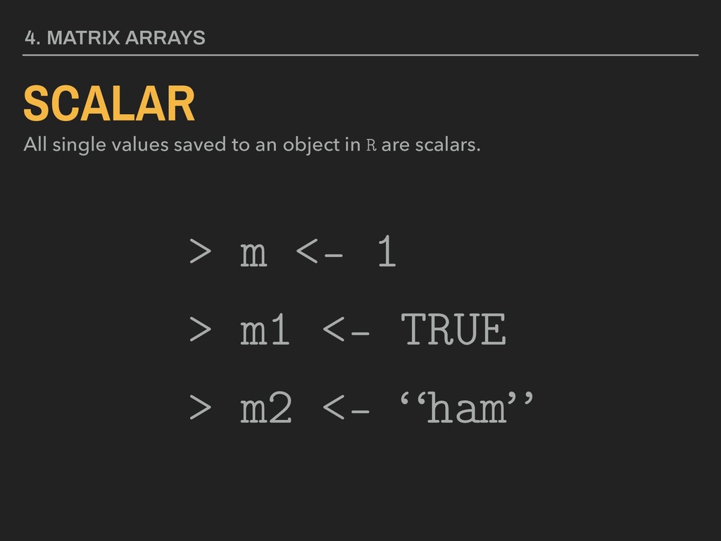
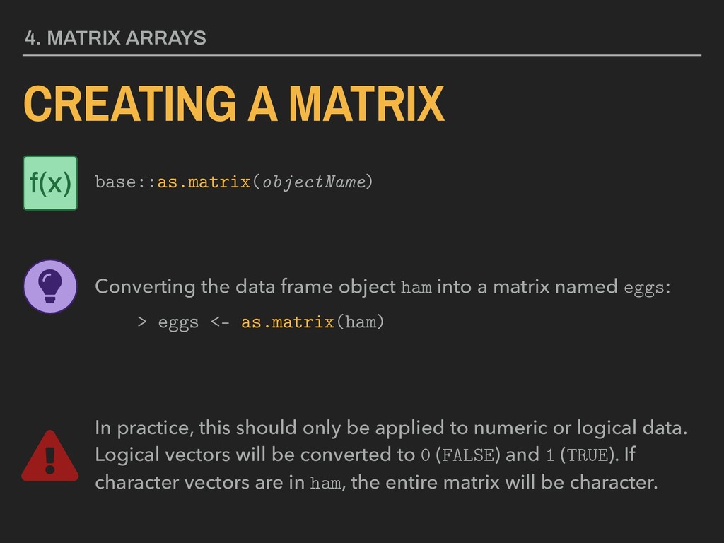
56. CREATING A MATRIX 4. MATRIX ARRAYS base::as.matrix(objectName) Converting the data frame object ham into a matrix named eggs: > eggs <- as.matrix(ham) In practice, this should only be applied to numeric or logical data. Logical vectors will be converted to 0 (FALSE) and 1 (TRUE). If character vectors are in ham, the entire matrix will be character. f(x)
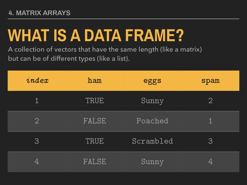
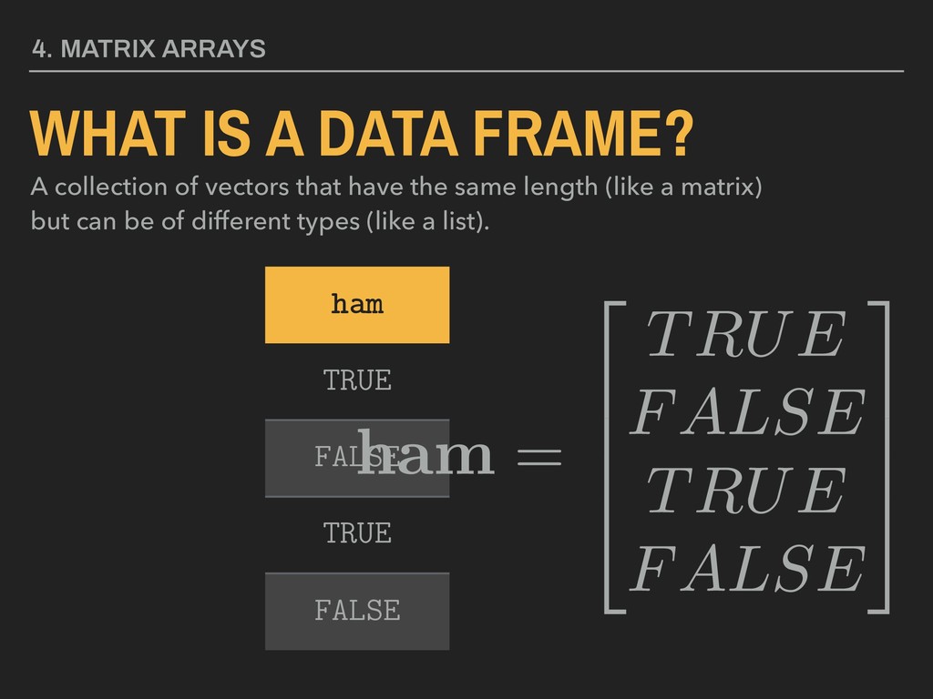
57. 4. MATRIX ARRAYS WHAT IS A DATA FRAME? A collection of vectors that have the same length (like a matrix)
 but can be of different types (like a list). index ham eggs spam 1 TRUE Sunny 2 2 FALSE Poached 1 3 TRUE Scrambled 3 4 FALSE Sunny 4
58. 4. MATRIX ARRAYS WHAT IS A DATA FRAME? A collection of vectors that have the same length (like a matrix)
 but can be of different types (like a list). ham TRUE FALSE TRUE FALSE
59. CREATING A DATA FRAME 4. MATRIX ARRAYS base::data.frame(vector, vector, stringsAsFactors = FALSE) Create an atomic vector of integers: > M <- data.frame(
 x = c(1, 2, 3),
 y = c(“a”, “b”, “a”),
 stringsAsFactors = FALSE) f(x)
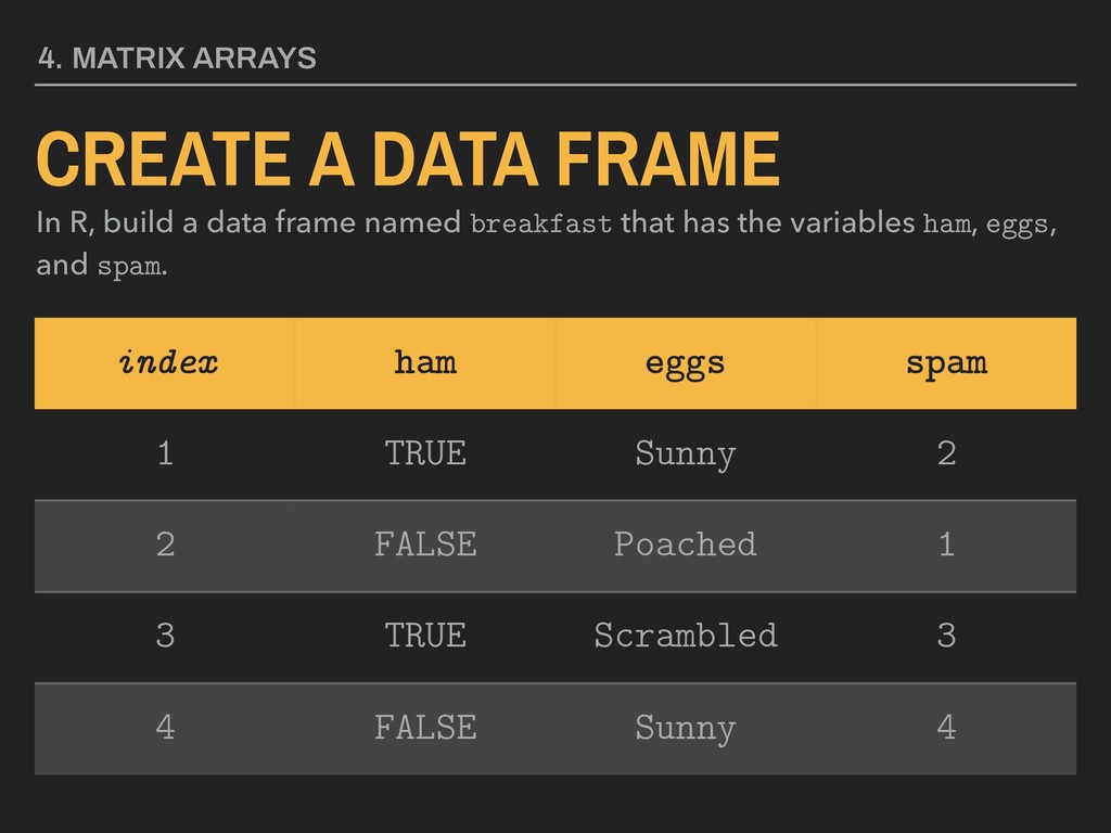
60. 4. MATRIX ARRAYS CREATE A DATA FRAME In R, build a data frame named breakfast that has the variables ham, eggs, and spam. index ham eggs spam 1 TRUE Sunny 2 2 FALSE Poached 1 3 TRUE Scrambled 3 4 FALSE Sunny 4
61. CREATE A DATA FRAME breakfast <- data.frame( ham = c(TRUE, FALSE, TRUE, FALSE), eggs = c(“Sunny”, “Poached”, “Scrambled”, “Sunny”), spam = c(2, 1, 3, 4), stringsAsFactors = FALSE) 4. MATRIX ARRAYS
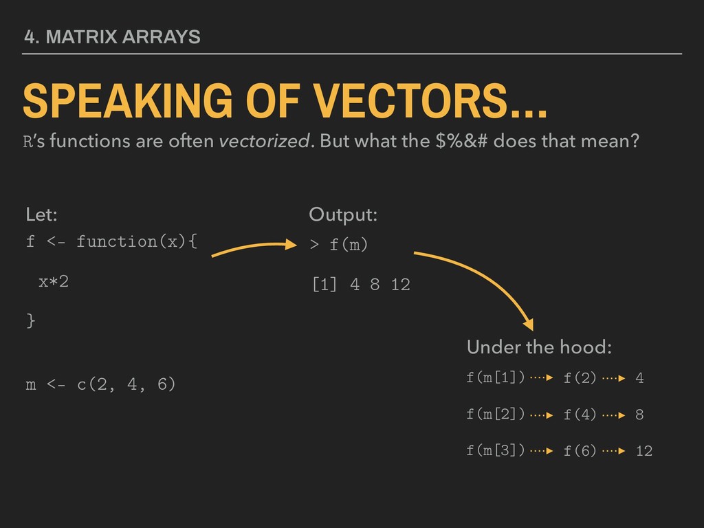
62. f(2) f(4) f(6) 4. MATRIX ARRAYS SPEAKING OF VECTORS… R’s functions are often vectorized. But what the $%&# does that mean? f <- function(x){ x*2 }
 m <- c(2, 4, 6) Let: Output: > f(m) [1] 4 8 12 f(m[1]) f(m[2]) f(m[3]) Under the hood: 4 8 12
63. CORRELATION IN R 5
64. 5. CORRELATION IN R MISSING DATA Missing data are represented by NA values in R. index ham eggs spam 1 TRUE Sunny 2 2 FALSE Poached 1 3 TRUE Scrambled NA 4 FALSE NA 4
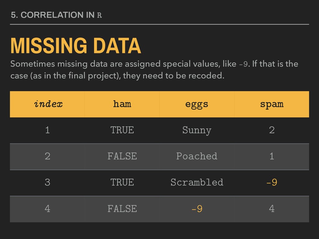
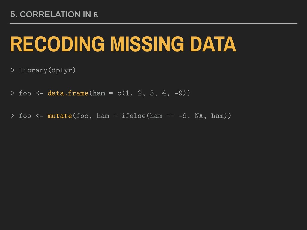
65. 5. CORRELATION IN R MISSING DATA Sometimes missing data are assigned special values, like -9. If that is the
 case (as in the final project), they need to be recoded. index ham eggs spam 1 TRUE Sunny 2 2 FALSE Poached 1 3 TRUE Scrambled -9 4 FALSE -9 4
66. RECODING MISSING DATA > library(dplyr) > foo <- data.frame(ham = c(1, 2, 3, 4, -9)) > foo <- mutate(foo, ham = ifelse(ham == -9, NA, ham)) 5. CORRELATION IN R
67. ▸ data is the data frame or tibble being used Available in naniar
 Download via CRAN 5. CORRELATION IN R MISSING DATA ANALYSIS Parameters: miss_var_summary(data) f(x)
68. ▸ data is the data frame or tibble being used 5. CORRELATION IN R MISSING DATA ANALYSIS Parameters: miss_var_summary(data) f(x)
69. MISSING DATA ANALYSIS 5. CORRELATION IN R miss_var_summary(data) f(x) Using from dplyr’s starwars data: miss_var_summary(starwars) Can be followed with %>% knitr::kable() to create a nicely formatted table of missing data.
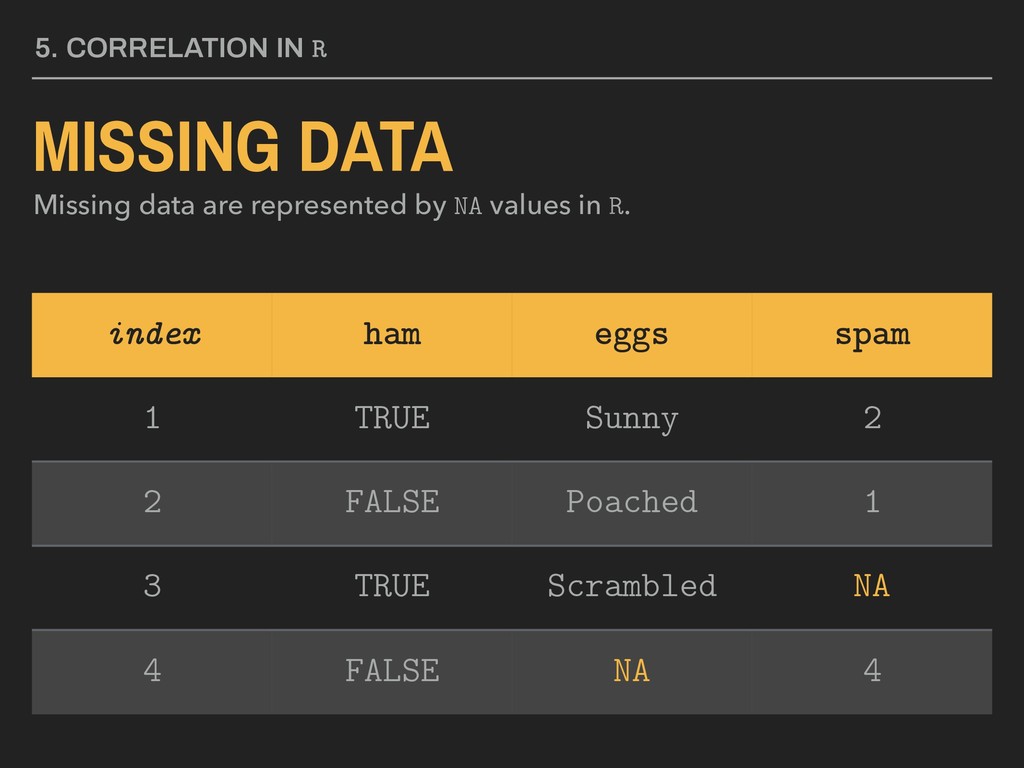
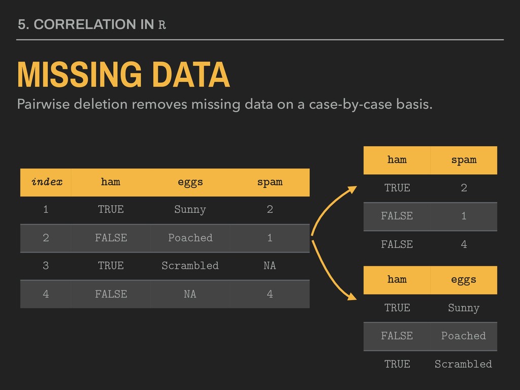
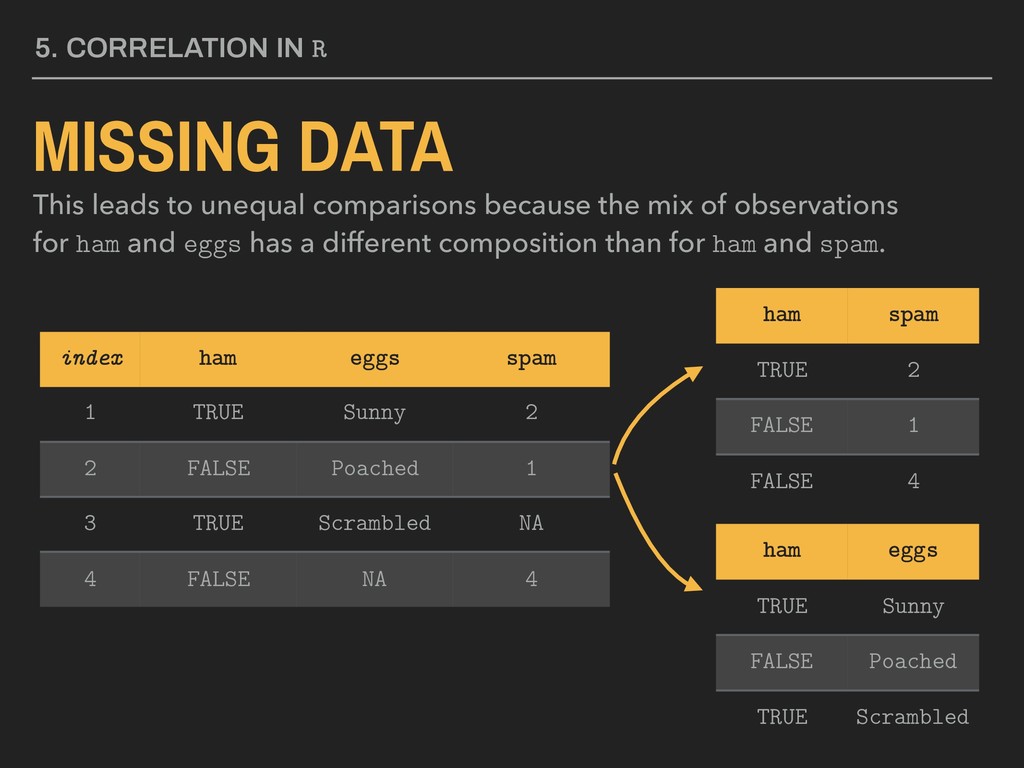
70. 5. CORRELATION IN R MISSING DATA Pairwise deletion removes missing data on a case-by-case basis. ham eggs TRUE Sunny FALSE Poached TRUE Scrambled ham spam TRUE 2 FALSE 1 FALSE 4 index ham eggs spam 1 TRUE Sunny 2 2 FALSE Poached 1 3 TRUE Scrambled NA 4 FALSE NA 4
71. 5. CORRELATION IN R MISSING DATA This leads to unequal comparisons because the mix of observations
 for ham and eggs has a different composition than for ham and spam. ham eggs TRUE Sunny FALSE Poached TRUE Scrambled ham spam TRUE 2 FALSE 1 FALSE 4 index ham eggs spam 1 TRUE Sunny 2 2 FALSE Poached 1 3 TRUE Scrambled NA 4 FALSE NA 4
72. 5. CORRELATION IN R MISSING DATA Listwise deletion removes all missing data for all given variables. index ham eggs spam 1 TRUE Sunny 2 2 FALSE Poached 1 3 TRUE Scrambled NA 4 FALSE NA 4
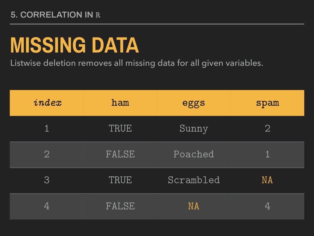
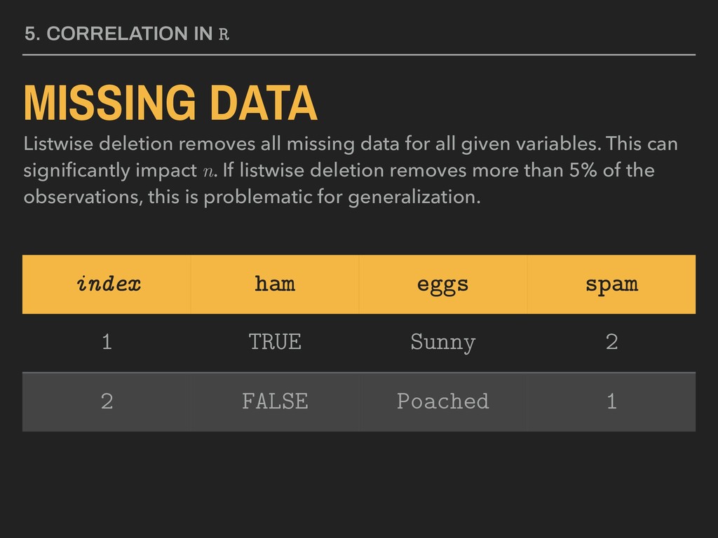
73. 5. CORRELATION IN R MISSING DATA Listwise deletion removes all missing data for all given variables. This can significantly impact n. If listwise deletion removes more than 5% of the observations, this is problematic for generalization. index ham eggs spam 1 TRUE Sunny 2 2 FALSE Poached 1
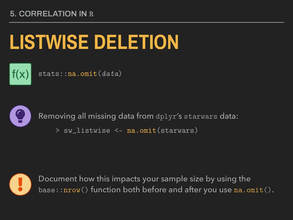
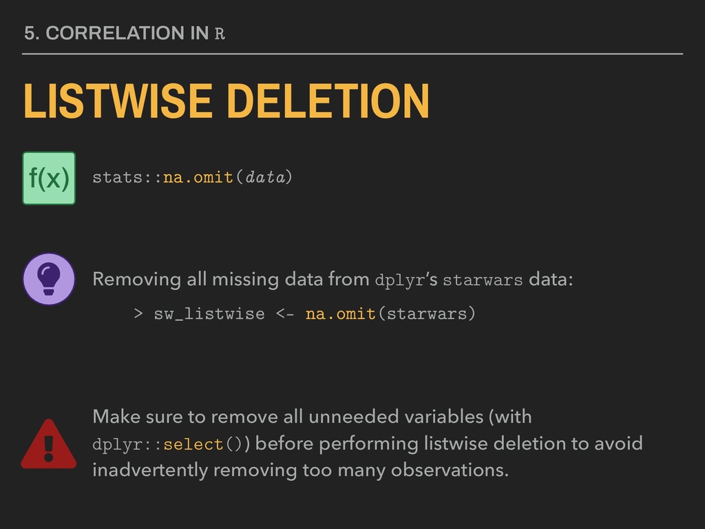
74. LISTWISE DELETION 5. CORRELATION IN R stats::na.omit(data) Removing all missing data from dplyr’s starwars data: > sw_listwise <- na.omit(starwars) Document how this impacts your sample size by using the base::nrow() function both before and after you use na.omit(). f(x)
75. LISTWISE DELETION 5. CORRELATION IN R stats::na.omit(data) Removing all missing data from dplyr’s starwars data: > sw_listwise <- na.omit(starwars) Make sure to remove all unneeded variables (with dplyr::select()) before performing listwise deletion to avoid inadvertently removing too many observations. f(x)
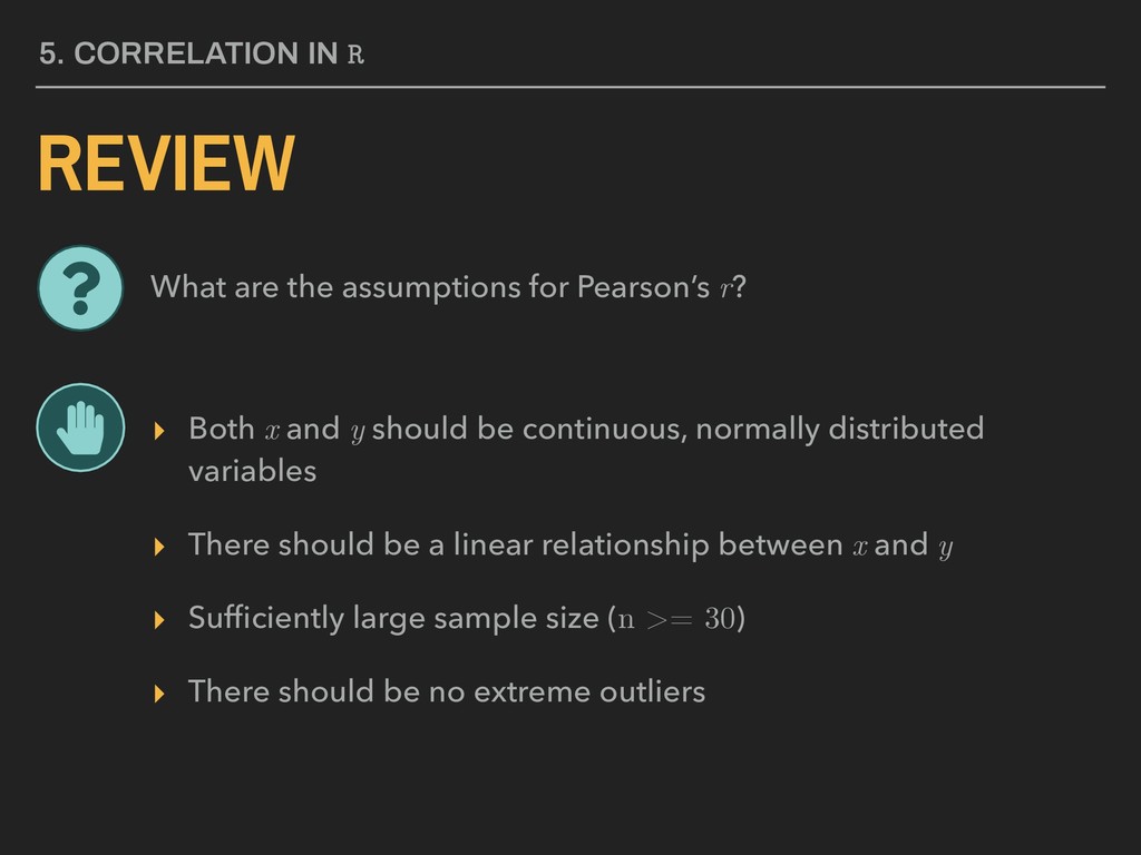
76. ? REVIEW ▸ Both x and y should be continuous, normally distributed variables ▸ There should be a linear relationship between x and y ▸ Sufficiently large sample size (n >= 30) ▸ There should be no extreme outliers 5. CORRELATION IN R What are the assumptions for Pearson’s r?
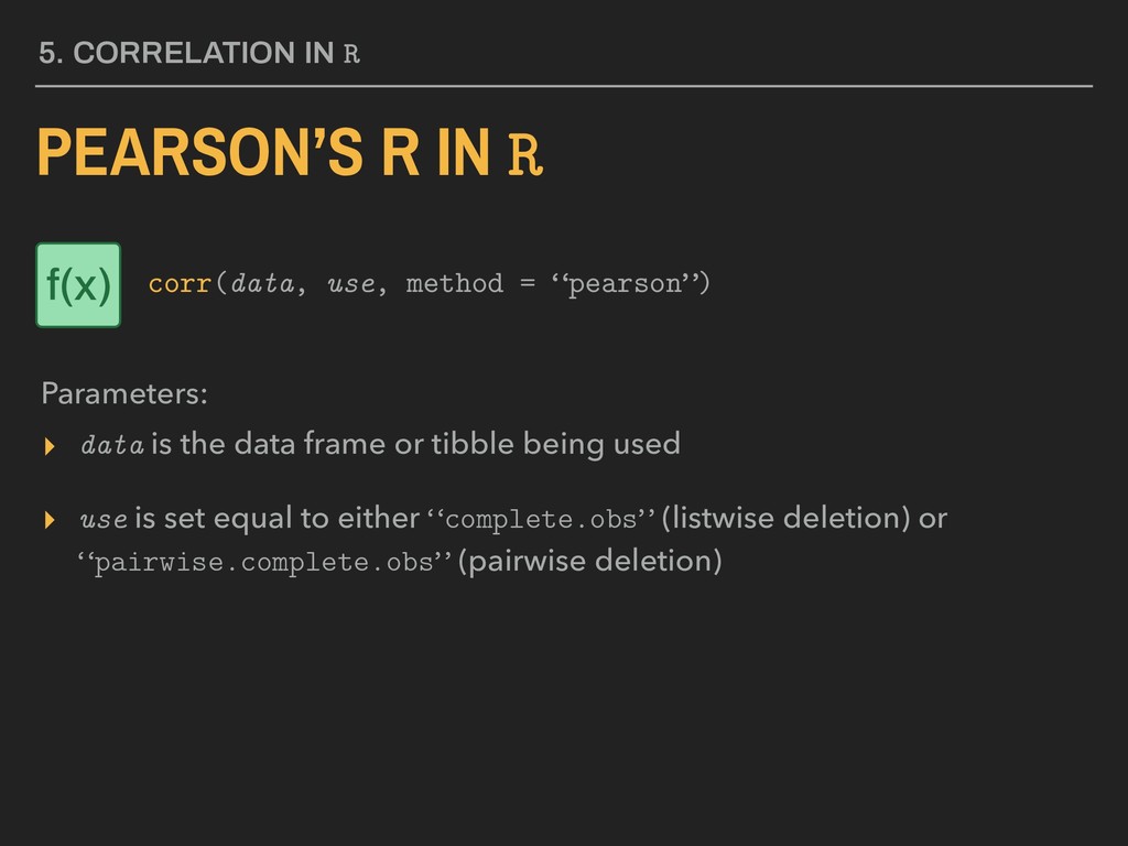
77. ▸ data is the data frame or tibble being used ▸ use is set equal to either “complete.obs” (listwise deletion) or “pairwise.complete.obs” (pairwise deletion) Available in stats
 Installed with base R 5. CORRELATION IN R PEARSON’S R IN R Parameters: corr(data, use, method = “pearson”) f(x)
78. ▸ data is the data frame or tibble being used ▸ use is set equal to either “complete.obs” (listwise deletion) or “pairwise.complete.obs” (pairwise deletion) 5. CORRELATION IN R PEARSON’S R IN R Parameters: corr(data, use, method = “pearson”) f(x)
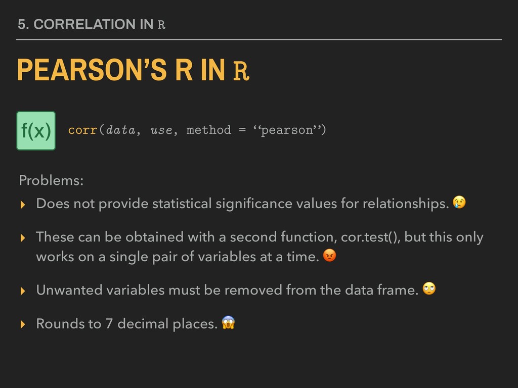
79. ▸ Does not provide statistical significance values for relationships. ▸ These can be obtained with a second function, cor.test(), but this only works on a single pair of variables at a time. ▸ Unwanted variables must be removed from the data frame. ▸ Rounds to 7 decimal places. 5. CORRELATION IN R PEARSON’S R IN R Problems: corr(data, use, method = “pearson”) f(x)
80. ▸ matrix is a matrix version of the data being used Available in Hmisc
 Download via CRAN 5. CORRELATION IN R PEARSON’S R IN R Parameters: rcorr(matrix, type = “pearson”) f(x)
81. ▸ matrix is a matrix version of the data being used 5. CORRELATION IN R PEARSON’S R IN R Parameters: rcorr(matrix, type = “pearson”) f(x)
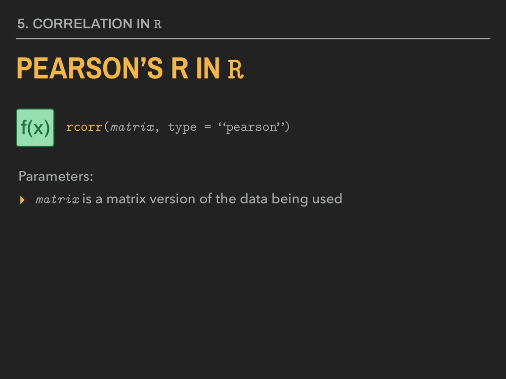
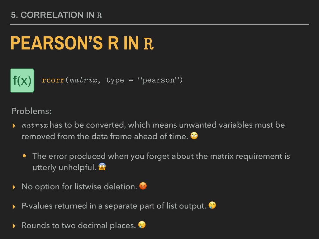
82. ▸ matrix has to be converted, which means unwanted variables must be removed from the data frame ahead of time. • The error produced when you forget about the matrix requirement is utterly unhelpful. ▸ No option for listwise deletion. ▸ P-values returned in a separate part of list output. ▸ Rounds to two decimal places. 5. CORRELATION IN R PEARSON’S R IN R Problems: rcorr(matrix, type = “pearson”) f(x)
83. SETUP FOR PEARSON’S R > library(dplyr) > library(ggplot2) > > autoData <- mpg > autoSubset <- select(autoData, cyl, cty, hwy) > autoSubset <- as.matrix(autoSubset) 5. CORRELATION IN R
84. PEARSON’S R IN R > rcorr(autoSubset, type = "pearson") cyl cty hwy cyl 1.00 -0.81 -0.76 cty -0.81 1.00 0.96 hwy -0.76 0.96 1.00 n= 234 P cyl cty hwy cyl 0 0 cty 0 0 hwy 0 0 5. CORRELATION IN R
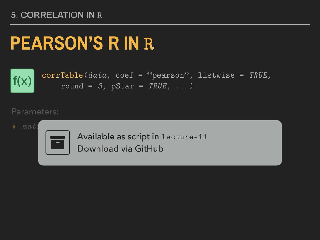
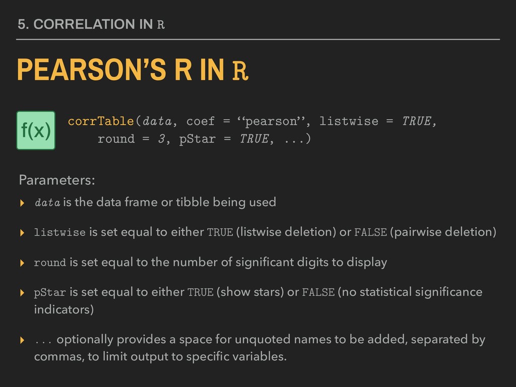
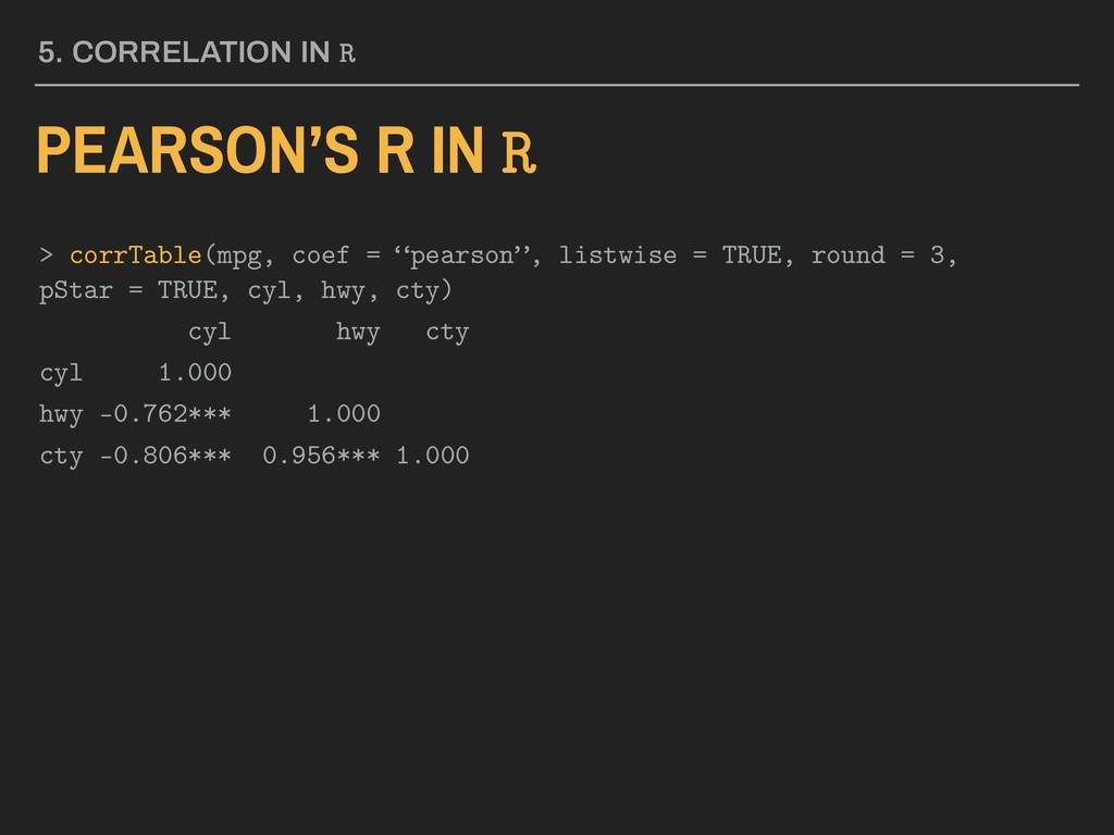
85. ▸ matrix is a matrix version of the data being used Available as script in lecture-11
 Download via GitHub 5. CORRELATION IN R PEARSON’S R IN R Parameters: corrTable(data, coef = “pearson”, listwise = TRUE,
 round = 3, pStar = TRUE, ...) f(x)
86. ▸ data is the data frame or tibble being used ▸ listwise is set equal to either TRUE (listwise deletion) or FALSE (pairwise deletion) ▸ round is set equal to the number of significant digits to display ▸ pStar is set equal to either TRUE (show stars) or FALSE (no statistical significance indicators) ▸ ... optionally provides a space for unquoted names to be added, separated by commas, to limit output to specific variables. 5. CORRELATION IN R PEARSON’S R IN R Parameters: corrTable(data, coef = “pearson”, listwise = TRUE,
 round = 3, pStar = TRUE, ...) f(x)
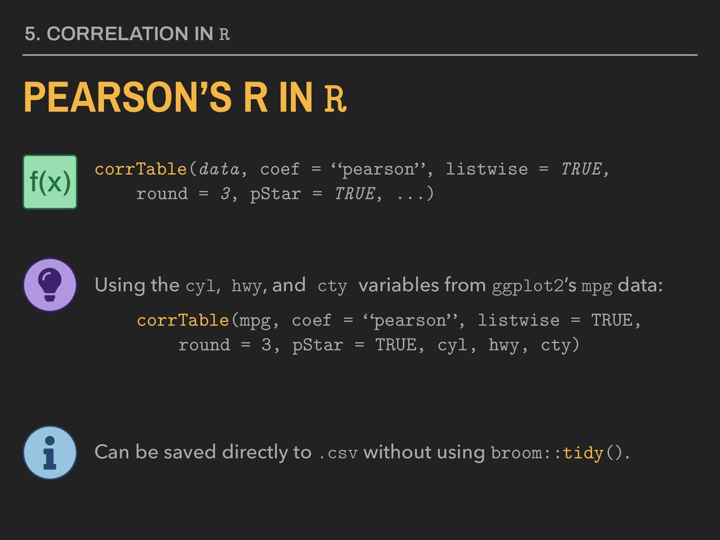
87. PEARSON’S R IN R 5. CORRELATION IN R corrTable(data, coef = “pearson”, listwise = TRUE,
 round = 3, pStar = TRUE, ...) Using the cyl, hwy, and cty variables from ggplot2’s mpg data: corrTable(mpg, coef = “pearson”, listwise = TRUE, round = 3, pStar = TRUE, cyl, hwy, cty) f(x) Can be followed with %>% knitr::kable() to create a nicely formatted table of correlation coefficients.
88. PEARSON’S R IN R 5. CORRELATION IN R corrTable(data, coef = “pearson”, listwise = TRUE,
 round = 3, pStar = TRUE, ...) Using the cyl, hwy, and cty variables from ggplot2’s mpg data: corrTable(mpg, coef = “pearson”, listwise = TRUE, round = 3, pStar = TRUE, cyl, hwy, cty) Can be saved directly to .csv without using broom::tidy(). f(x)
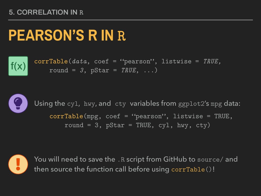
89. PEARSON’S R IN R 5. CORRELATION IN R corrTable(data, coef = “pearson”, listwise = TRUE,
 round = 3, pStar = TRUE, ...) Using the cyl, hwy, and cty variables from ggplot2’s mpg data: corrTable(mpg, coef = “pearson”, listwise = TRUE, round = 3, pStar = TRUE, cyl, hwy, cty) You will need to save the .R script from GitHub to source/ and then source the function call before using corrTable()! f(x)
90. PEARSON’S R IN R > corrTable(mpg, coef = “pearson”, listwise = TRUE, round = 3, 
 pStar = TRUE, cyl, hwy, cty) cyl hwy cty cyl 1.000 hwy -0.762*** 1.000 cty -0.806*** 0.956*** 1.000 5. CORRELATION IN R
91. POWER ANALYSES FOR CORRELATION 6
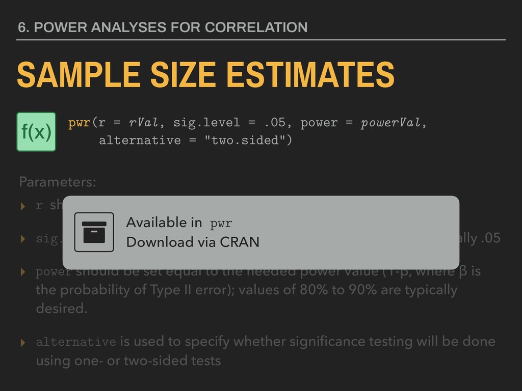
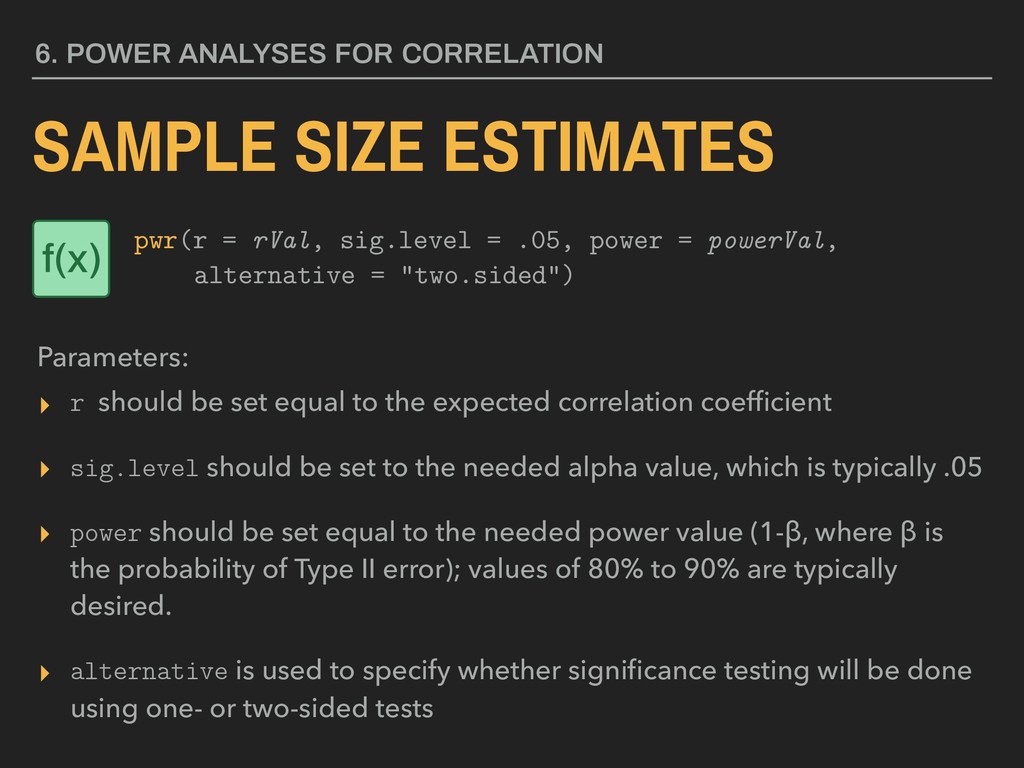
92. ▸ r should be set equal to the expected correlation coefficient ▸ sig.level should be set to the needed alpha value, which is typically .05 ▸ power should be set equal to the needed power value (1-β, where β is the probability of Type II error); values of 80% to 90% are typically desired. ▸ alternative is used to specify whether significance testing will be done using one- or two-sided tests Available in pwr
 Download via CRAN 6. POWER ANALYSES FOR CORRELATION SAMPLE SIZE ESTIMATES Parameters: pwr(r = rVal, sig.level = .05, power = powerVal, alternative = "two.sided") f(x)
93. ▸ r should be set equal to the expected correlation coefficient ▸ sig.level should be set to the needed alpha value, which is typically .05 ▸ power should be set equal to the needed power value (1-β, where β is the probability of Type II error); values of 80% to 90% are typically desired. ▸ alternative is used to specify whether significance testing will be done using one- or two-sided tests 6. POWER ANALYSES FOR CORRELATION SAMPLE SIZE ESTIMATES Parameters: pwr(r = rVal, sig.level = .05, power = powerVal, alternative = "two.sided") f(x)
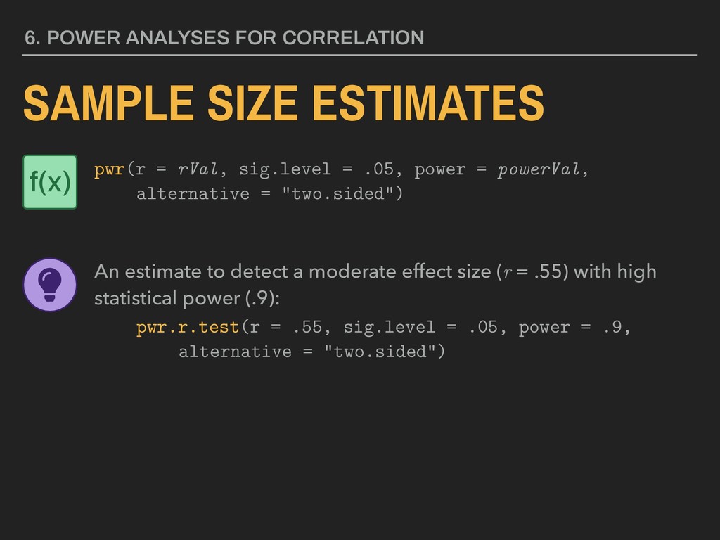
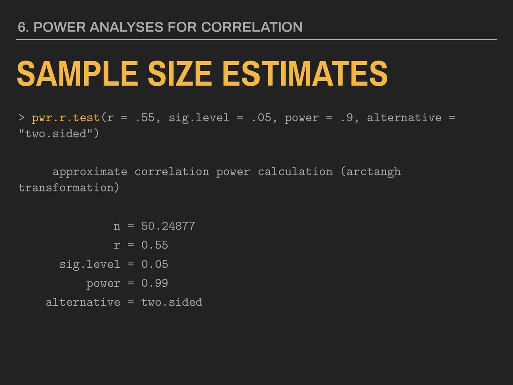
94. SAMPLE SIZE ESTIMATES 6. POWER ANALYSES FOR CORRELATION pwr(r = rVal, sig.level = .05, power = powerVal, alternative = "two.sided") An estimate to detect a moderate effect size (r = .55) with high statistical power (.9): pwr.r.test(r = .55, sig.level = .05, power = .9, alternative = "two.sided") f(x)
95. SAMPLE SIZE ESTIMATES > pwr.r.test(r = .55, sig.level = .05, power = .9, alternative = "two.sided") approximate correlation power calculation (arctangh transformation) n = 50.24877 r = 0.55 sig.level = 0.05 power = 0.99 alternative = two.sided 6. POWER ANALYSES FOR CORRELATION
96. 7 BACK 
 MATTER
97. AGENDA REVIEW 7. BACK MATTER 2. More with knitr 3. Scatterplots 4. Matrix Arrays 5. Correlation in R 6. Power Analyses for Correlation
98. Reminder - no additional lecture preps! REMINDERS 7. BACK MATTER Draft papers due next Monday! Lab 10 and Problem Set 05 due next Monday as is peer review of partner’s materials!