Designing for colorblindness with colorblindr

Talk on our new R package colorblindr, which simulates color vision deficiencies on ggplots and images.
https://github.com/clauswilke/colorblindr

Transcript

1. colorblindr Claire McWhite & Claus Wilke R Users Meetup 9/5/2017
2. Color vision deficiencies
3. Why design for colorblindness? • In some populations, up to 10% of men are have color vision deficiencies (cvd) • Any medium-size audience of people is very likely to have someone with color vision deficiencies
4. Rules from just one person with deutanomaly • Forbidden combinations: • No red/black (if lines too small) • No pink/grey/some light blues • No purple/blue • No orange/yellow • Rules • Skinny lines much harder to distinguish than blocks of color • Makes data points bigger • No using the default ggplot color scheme
5. Wishlist for a colorblindness sim for ggplot • Be able to replace colors on existing plots and images • Use most up-to-date models of color vision deficiencies • “A Physiologically-based Model for Simulation of Color Vision Deficiency”, Machado 2009
7. How does it work? • Loop through grob tree to find color attributes • Convert all color codes to RGB, then apply RGB transform matrix. 0.203876 0.990338 -0.194214 0.112975 0.794542 0.092483 -0.005222 0.041043 1.046265 Transform matrix for a severe protanomaly
8. > p <- ggplot(iris, aes(x=Sepal.Width, y=Sepal.Length, color=Species)) + geom_point()
9. > cvd_grid(p) `cvd_grid` is a convenience function for quickly showing the most severe forms of each color vision deficiency.
10.  p2 <- edit_colors(p, deutan, sev=0.7)  plot_grid(p,p2) Main function `edit_colors`.
11. > library(magick) > p <- ggdraw() + draw_image(“cell.jpg") > plot_grid(p)
12. Deutan Protan Tritan Monochrome > cvd_grid(p)
13. > view_cvd(p)
14. Recently, NOAA added a new color category for rainfall totals around Houston The most extreme value ‘pink’ is equivalent the ocean color for the most common forms of colorblindness
15. > view_cvd(p)
16. > p + scale_fill_okabeIto Use color scales designed for cvds Okabe & Ito: “Color Universal Design (CUD) ” http://jfly.iam.u-tokyo.ac.jp/color/
17. Other uses • colorblindr turns out to be simple way easy way to recolor images
18. > p <- ggplot(iris, aes(Sepal.Width, fill=Species)) + geom_density(alpha = 0.7) > to_white <- function(c) {"#FFFFFF"} # convert everything to white > to_black <- function(c) {"#000000"} # convert everything to black > p2 <- edit_colors(p, colfun = to_white, fillfun = to_black) > p3 <- edit_colors(p, colfun = to_black, fillfun = to_white) > plot_grid(p, p2, p3, ncol=1) Custom recoloring
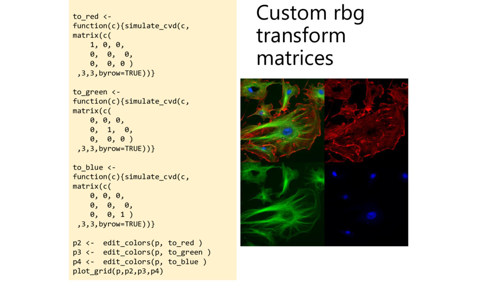
19. Custom rbg transform matrices to_red <- function(c){simulate_cvd(c, matrix(c( 1, 0, 0, 0, 0, 0, 0, 0, 0 ) ,3,3,byrow=TRUE))} to_green <- function(c){simulate_cvd(c, matrix(c( 0, 0, 0, 0, 1, 0, 0, 0, 0 ) ,3,3,byrow=TRUE))} to_blue <- function(c){simulate_cvd(c, matrix(c( 0, 0, 0, 0, 0, 0, 0, 0, 1 ) ,3,3,byrow=TRUE))} p2 <- edit_colors(p, to_red ) p3 <- edit_colors(p, to_green ) p4 <- edit_colors(p, to_blue ) plot_grid(p,p2,p3,p4)
20. New figure/image design workflow • Make image • Check colors using `cvd_grid` • Iterate color choices until colors are distinguishable in all conditions
21. Check out github.com/clauswilke/colorblindr
22. Okabe & Ito: “Color Universal Design (CUD) ” http://jfly.iam.u-tokyo.ac.jp/color/