Causal: Week 3

Transcript

1. S , , . William Lowe Hertie School th September
2. L Last we thought about external validity and randomized controlled trials is week we’ll think about the observational studies and ask three questions: → Can I get a representative estimate from a representative sample? → What should I control for? (Number will surprise you) → And how should I interpret the results?
3. W FDI -2.5 0.0 2.5 5.0 7.5 FDI
4. F Does being more democratic lead to more FDI? According to Jensen ( ), yes. We’ll look at a (simpli ed) version of his time series cross-sectional analysis → Worldwide (but with some missingness) → years of annual data: - → Regime on a point scale (higher, more democratic) → Controls for lots of potential confounders, predictors of FDI, and country xed e ects → tl;dr small but signi cant positive e ect of regime time on FDI
5. F Regime type is a continuous treatment, so we’ll think of the causal e ect of regime type as → the di erence in expected FDI for an exogenous one unit increase in regime measure Substantive question: → Do we think the e ect of regime is the same on FDI everywhere? If not, we expect heterogenous treatment e ects → though we can still hope that regression will give us an ATE
6. T : B Possibly heterogenous additive treatment e ects τi and su cient covariates X: Yi = Yi + τi Xi (Y , τ) ⊥ ⊥ X Z e average treatment e ect is ATE = E[τi ] = E[Yi − Yi ] Jensen ts his favourite OLS regression model, controlling for all the Zs Yi = β + Xi βX + Zi βZ + єi What are we estimating with βX with OLS?
7. C If τi = τ then ATE = βX Just as we hoped. If τi ≠ τ, that is: the treatment e ects vary by case, then it’s more interesting.
8. C If τi = τ then ATE = βX Just as we hoped. If τi ≠ τ, that is: the treatment e ects vary by case, then it’s more interesting. Consider a di erent regression, predicting X using Z Xi = γ + ZiγZ + η If X is binary then E[X Z] = p(Z) is the propensity score.
9. H Now de ne a weight w(Zi ) for each case w(Zi ) = (Xi − E[Xi Zi ]) is weight is large when it’s unpredictable from the covariates what the treatment status of the case will be, e.g. → If treatment is binary, it’s largest when w(Zi ) = . → For Jensen, it’s when the residuals are large e expected (average) value of this weight is the variance of treatment assignment given Z. E[w(Zi )] = Var[Xi Zi ] Finally, notice that the weights have nothing to do with outcomes.
10. H Why would we care about these weights? Because we can show (Aronow & Samii, ) that the regression coe cient we would like to be the ATE is β = E[w(Zi )τi ] E[w(Zi )]
11. H Why would we care about these weights? Because we can show (Aronow & Samii, ) that the regression coe cient we would like to be the ATE is β = E[w(Zi )τi ] E[w(Zi )] For randomized experiments, we may not care much because β = E[w(Zi )τi ] E[w(Zi )] = E[w(Zi )]E[τi ] E[w(Zi )] = E[τi ] But for observational studies with varying treatment e ects → Some cases matter a lot more than others
12. N
13. H 0.01 0.02 0.03 0.04 0.05 0.06 OLS weights
14. L 0.001 0.002 0.003 0.004 0.005 0.006 OLS weights
15. L Haiti Honduras Russian Federation South Africa Yemen, Rep. Albania Benin Central African Republic Congo, Rep. Germany 1980 1990 1980 1990 1980 1990 1980 1990 1980 1990 -6 -4 -2 0 2 -6 -4 -2 0 2 year Fvar5 5 10 15 regime
16. L Countries that have few observations → Not much opportunity for variation → Well predicted by xed e ects, e.g. Germany We have to hope that the treatment e ects here are negligible (or the same as elsewhere)
17. H Peru Philippines Poland Uruguay Zimbabwe Argentina Hungary Madagascar Niger Pakistan 1980 1990 1980 1990 1980 1990 1980 1990 1980 1990 0.0 2.5 5.0 7.5 10.0 0.0 2.5 5.0 7.5 10.0 year Fvar5 5 10 15 regime
18. H Countries that have plenty of observations → Variation in regime and FDI → Badly predicted by country xed e ects In this period there is a steady upward (democratic) trend in regime measures. Also in FDI... → We might want to worry about that. But not now and not here.
19. M It feels like regression on representative samples ought to get us externally valid results... → Alas, not necessarily
20. M It feels like regression on representative samples ought to get us externally valid results... → Alas, not necessarily Estimates from a randomized experiment are only directly informative for the subpopula- tion whose treatment status can be manipulated by the investigator. Estimates from an observational study can only be directly informative for the subpopula- tion that exhibits some unpredictability in their treatment status a er accounting for control variables. (Aronow & Samii, )
21. A So, would this weighting happen if I used matching instead? No, but you’d get a di erent weighting. → Regression: averaged over Z with weights proportional to treatment variance given the control variables → Matching, e.g. for the ATT: averaged over Z with weights proportional to the probability of being treated at that level of Z → Case less likely to be treated? Smaller weight
22. M , R , . And back in Germany: No variation, so zero weight → As far as regression can tell, there is no possibility of regime change in Germany (because there’s none in the data) → Assumption: Positivity fails / the counterfactual does not exist More detailed comparison in ch. . of Angrist and Pischke ( ) and a slightly more general framework in Hirano et al. ( )
24. C Cinelli et al. ( ) o er a typology of good and bad controls → Let’s take a quick look Much of this you already know, some perhaps not...
25. C
26. M !
27. -
28. D
29. ...
30. D ’
33. Wait, what? How could this be bad? → It can make confounding worse (Middleton et al., ; Wooldridge, )
34. B Here’s a linear version with each e ect marked (Pearl, ) X Z Y A α β γ γ
35. B Here’s a linear version with each e ect marked (Pearl, ) X Z Y A α β γ γ Compare the causal e ect to some observational quantities τ = E[YX= − YX= ] = β τnaive = E[Y X = ] − E[Y X = ] = β + γ γ τA = E[Y X = , A] − E[Y X = , A] = β + γ γ − α
37. C Which of these coe cients is causally interpretable? (Keele et al., )
38. C Public service announcement: → You can’t generally interpret the coe cients of control variables causally
39. C Public service announcement: → You can’t generally interpret the coe cients of control variables causally It’s a very popular thing to do (H¨ unermund & Louw, ), but → ‘It is worth noting the results of our control variables’ (It’s not) → Nobody cares about their signs being ‘in the expected direction’
40. O Can I get a representative estimate from a representative sample? → Sometimes? But now you know what it does behind the curtain What should I control for in my research? → Now we’ve got a list And how should I interpret the results (of controlling for things) → You shouldn’t. See, causal inference makes some things easier...
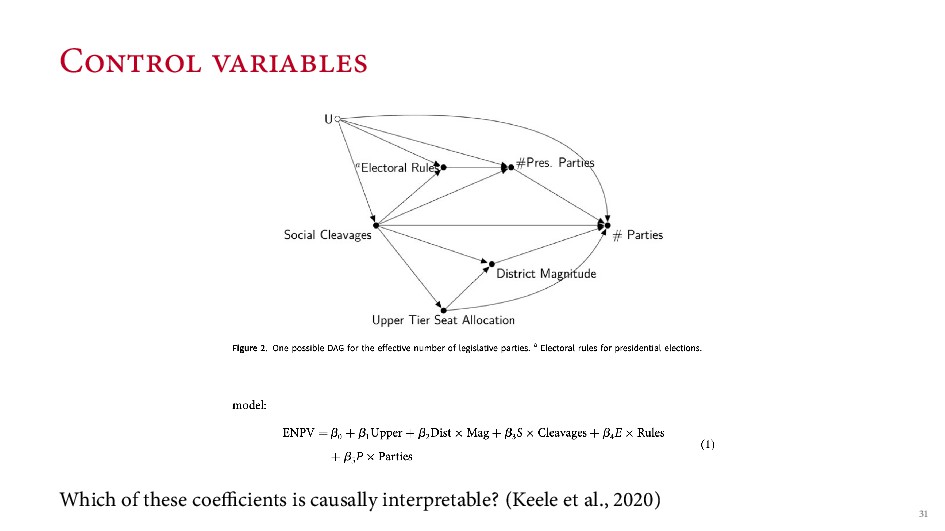
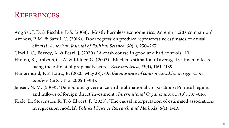
41. R Angrist, J. D. & Pischke, J.-S. ( ). ‘Mostly harmless econometrics: An empiricists companion’. Aronow, P. M. & Samii, C. ( ). ‘Does regression produce representative estimates of causal e ects?’ American Journal of Political Science, ( ), – . Cinelli, C., Forney, A. & Pearl, J. ( ). ‘A crash course in good and bad controls’. . Hirano, K., Imbens, G. W. & Ridder, G. ( ). ‘E cient estimation of average treatment e ects using the estimated propensity score’. Econometrica, ( ), – . H¨ unermund, P. & Louw, B. ( , May ). On the nuisance of control variables in regression analysis (arXiv No. . ). Jensen, N. M. ( ). ‘Democratic governance and multinational corporations: Political regimes and in ows of foreign direct investment’. International Organization, ( ), – . Keele, L., Stevenson, R. T. & Elwert, F. ( ). ‘The causal interpretation of estimated associations in regression models’. Political Science Research and Methods, ( ), – .
42. R Middleton, J. A., Scott, M. A., Diakow, R. & Hill, J. L. ( ). ‘Bias ampli cation and bias unmasking’. Political Analysis, ( ), – . Pearl, J. ( ). ‘On a class of bias-amplifying variables that endanger e ect estimates’. Proceedings of the Twenty-Sixth Conference on Uncertainty in Arti cial Intelligence, – . Wooldridge, J. M. ( ). ‘Should instrumental variables be used as matching variables?’ Research in Economics, ( ), – .