ree broad normative possibilities → Represent all uncertainty with probability (Bayesian statistics) → Represent uncertainty due to random processes with probabilities (Classical statistics, ‘frequentism’) → Probability is not used to represent uncertainty (qualitative research?) And two broad applications → As a model of an ideal decision maker → As a tool for statistical inference and data science
is the object? Applications ML and data science Getting some intuition for Bayesian updating How to be unsure How to be wrong How to deal with big problems Computation! and probability theory in easy mode How to be wrong again
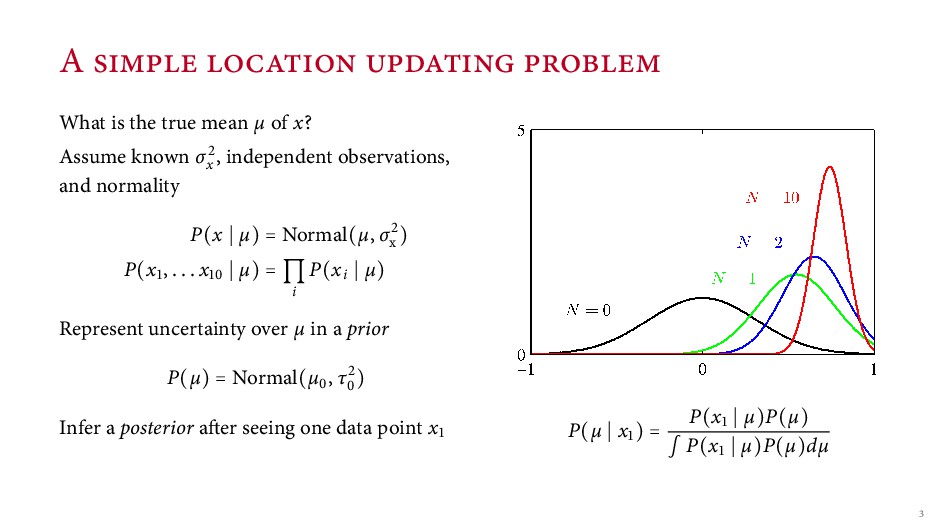
known σx , independent observations, and normality P(x µ) = Normal(µ, σx ) P(x , . . . x µ) = i P(xi µ) Represent uncertainty over µ in a prior P(µ) = Normal(µ , τ ) Infer a posterior a er seeing one data point x P(µ x ) = P(x µ)P(µ) ∫ P(x µ)P(µ)dµ
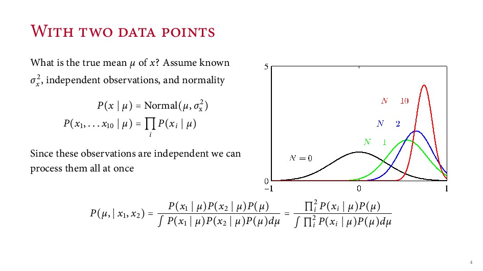
known σx , independent observations, and normality P(x µ) = Normal(µ, σx ) P(x , . . . x µ) = i P(xi µ) Since these observations are independent we can process them all at once P(µ, x , x ) = P(x µ)P(x µ)P(µ) ∫ P(x µ)P(x µ)P(µ)dµ = ∏i P(xi µ)P(µ) ∫ ∏i P(xi µ)P(µ)dµ
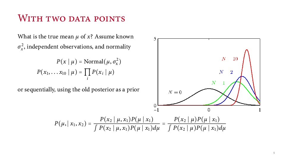
known σx , independent observations, and normality P(x µ) = Normal(µ, σx ) P(x , . . . x µ) = i P(xi µ) or sequentially, using the old posterior as a prior P(µ, x , x ) = P(x µ, x )P(µ x ) ∫ P(x µ, x )P(µ x )dµ = P(x µ)P(µ x ) ∫ P(x µ)P(µ x )dµ
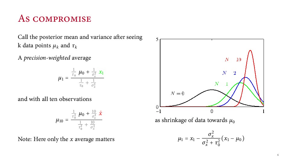
k data points µk and τk A precision-weighted average µ = τ µ + σx x τ + σx and with all ten observations µ = τ µ + σx ¯ x τ + σx Note: Here only the x average matters as shrinkage of data towards µ µ = x − σx σx + τ (x − µ )
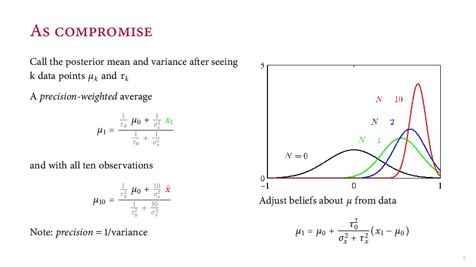
k data points µk and τk A precision-weighted average µ = τ µ + σx x τ + σx and with all ten observations µ = τ µ + σx ¯ x τ + σx Note: precision = /variance Adjust beliefs about µ from data µ = µ + τ σx + τx (x − µ )
Keep everything the same as before but let P(µ(t+ ) µ(t)) = Normal(µ(t), σµ) en the adjustment to our posterior over µ is slightly more complicated, but the mean still has the form µt = µt− + K (xt− − µt− ) where K is a ‘gain’ that weights the ‘observation error’ or ‘innovation’ at t is is a lter (speci cally, a Kalman Filter) but also an implementation of Bayesian updating for the simplest linear normal state space model
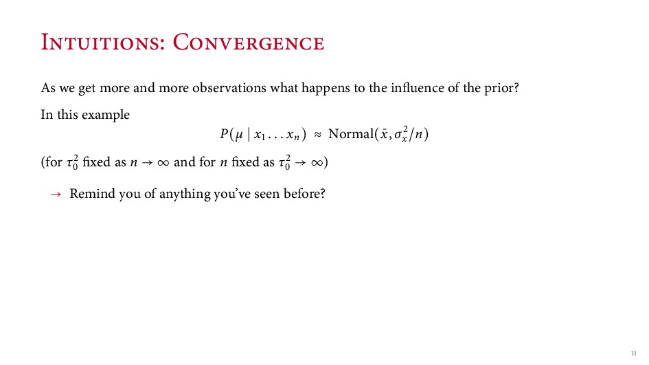
what happens to the in uence of the prior? In this example P(µ x . . . xn) ≈ Normal(¯ x, σx n) (for τ xed as n → ∞ and for n xed as τ → ∞) → Remind you of anything you’ve seen before?
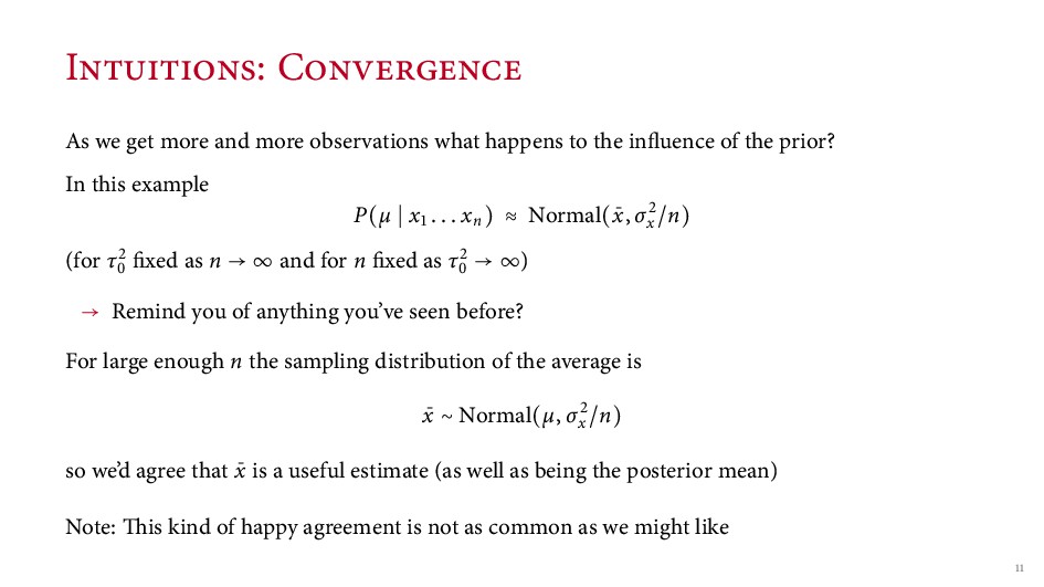
what happens to the in uence of the prior? In this example P(µ x . . . xn) ≈ Normal(¯ x, σx n) (for τ xed as n → ∞ and for n xed as τ → ∞) → Remind you of anything you’ve seen before? For large enough n the sampling distribution of the average is ¯ x ∼ Normal(µ, σx n) so we’d agree that ¯ x is a useful estimate (as well as being the posterior mean) Note: is kind of happy agreement is not as common as we might like
what happens to the in uence of the prior? In this example P(µ x . . . xn) ≈ Normal(¯ x, σx n) (for τ xed as n → ∞ and for n xed as τ → ∞) → Remind you of anything you’ve seen before? For large enough n the sampling distribution of the average is ¯ x ∼ Normal(µ, σx n) so we’d agree that ¯ x is a useful estimate (as well as being the posterior mean) Note: is kind of happy agreement is not as common as we might like
atness A subtle problem with the original idea → Flatness can be relative to parameterization Example: → How e ective is a new drug? Possible parameterizations → Probability of e ectiveness: π → Odds of being e ectiveness: π ( − π) → Logit of e ectiveness: log(π ( − π))
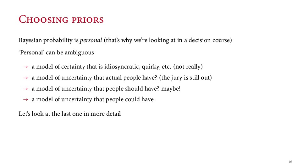
in a decision course) ‘Personal’ can be ambiguous → a model of certainty that is idiosyncratic, quirky, etc. (not really) → a model of uncertainty that actual people have? (the jury is still out) → a model of uncertainty that people should have? maybe! → a model of uncertainty that people could have Let’s look at the last one in more detail
‘edge’ of the prior support closest to truth... may not be very reassuring We can be redeemably and irredeemably wrong → Prior is bad but (eventually) data will brings us to the truth → Prior is bad and we cannot get there from here More on the applications consequences of this later...
→ What about really big models, e.g. neural networks, decision tree. Or di cult decision problems? Complicated models present several challenges → Finding sensible priors for parameters → Dealing with ‘nuisance’ parameters → Working with intractable posteriors Let’s take a closer look at the last two
→ What about really big models, e.g. neural networks, decision tree. Or di cult decision problems? Complicated models present several challenges → Finding sensible priors for parameters → Dealing with ‘nuisance’ parameters → Working with intractable posteriors Let’s take a closer look at the last two Earlier we assumed we knew σx → What if we don’t?
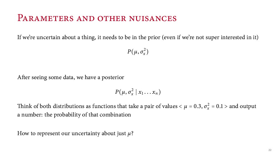
be in the prior (even if we’re not super interested in it) P(µ, σx ) A er seeing some data, we have a posterior P(µ, σx x . . . xn) ink of both distributions as functions that take a pair of values < µ = . , σx = . > and output a number: the probability of that combination How to represent our uncertainty about just µ?
. . xn) = P(µ, σx x . . . xn)dσx a.k.a. just sum over the things you don’t care about Not to be mistaken for choosing some σx = s and looking at P(µ, σx , x . . . xn) Note: the tails of this distribution are fatter (and not Normal) when we don’t know σ
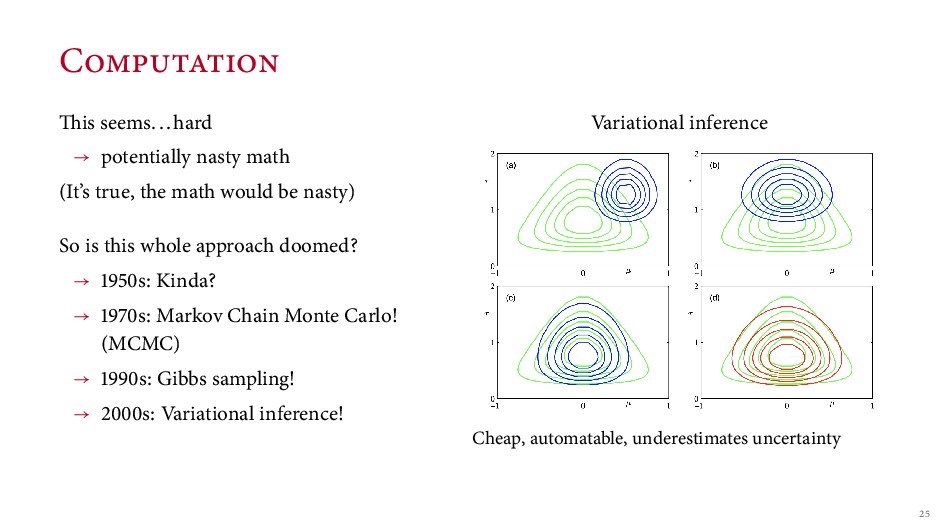
math would be nasty) So is this whole approach doomed? → s: Kinda? → s: Markov Chain Monte Carlo! (MCMC) → s: Gibbs sampling! → s: Variational inference! Variational inference Cheap, automatable, underestimates uncertainty
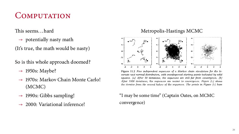
math would be nasty) So is this whole approach doomed? → s: Maybe? → s: Markov Chain Monte Carlo! (MCMC) → s: Gibbs sampling! → : Variational inference! Metropolis-Hastings MCMC “I may be some time” (Captain Oates, on MCMC convergence)
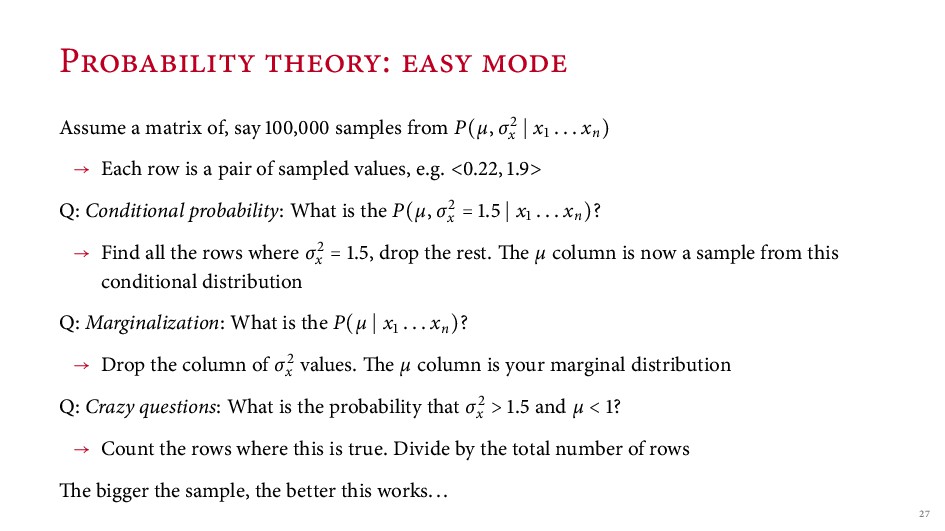
P(µ, σx x . . . xn) → Each row is a pair of sampled values, e.g. < . , . > Q: Conditional probability: What is the P(µ, σx = . x . . . xn)? → Find all the rows where σx = . , drop the rest. e µ column is now a sample from this conditional distribution
P(µ, σx x . . . xn) → Each row is a pair of sampled values, e.g. < . , . > Q: Conditional probability: What is the P(µ, σx = . x . . . xn)? → Find all the rows where σx = . , drop the rest. e µ column is now a sample from this conditional distribution Q: Marginalization: What is the P(µ x . . . xn)? → Drop the column of σx values. e µ column is your marginal distribution
P(µ, σx x . . . xn) → Each row is a pair of sampled values, e.g. < . , . > Q: Conditional probability: What is the P(µ, σx = . x . . . xn)? → Find all the rows where σx = . , drop the rest. e µ column is now a sample from this conditional distribution Q: Marginalization: What is the P(µ x . . . xn)? → Drop the column of σx values. e µ column is your marginal distribution Q: Crazy questions: What is the probability that σx > . and µ < ? → Count the rows where this is true. Divide by the total number of rows
P(µ, σx x . . . xn) → Each row is a pair of sampled values, e.g. < . , . > Q: Conditional probability: What is the P(µ, σx = . x . . . xn)? → Find all the rows where σx = . , drop the rest. e µ column is now a sample from this conditional distribution Q: Marginalization: What is the P(µ x . . . xn)? → Drop the column of σx values. e µ column is your marginal distribution Q: Crazy questions: What is the probability that σx > . and µ < ? → Count the rows where this is true. Divide by the total number of rows e bigger the sample, the better this works...
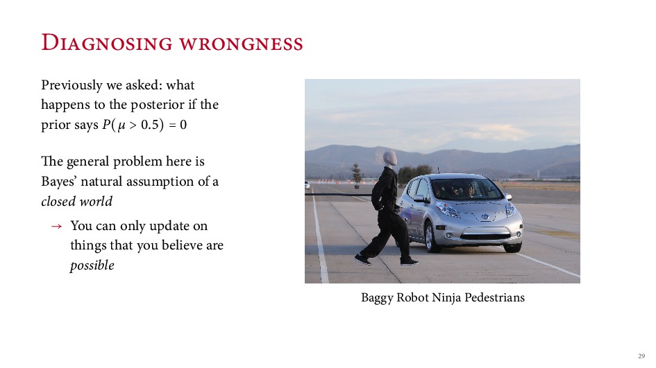
the prior says P(µ > . ) = e general problem here is Bayes’ natural assumption of a closed world → You can only update on things that you believe are possible Baggy Robot Ninja Pedestrians
put probability on things that were sampled / randomized / could have gone di erently / non-mental → Generate estimators (procedures with guarantees, not distributions with properties) → Test hypotheses, o en (Fisher) with unstated alternatives Oh hai
for predictions Calibration (for classi ers): → If a classi er says: P(recidivism)= . then ≈ % of people predicted to recidivize(?) do so Bayes does not, in general, guarantee this
Expressing serious uncertain is harder that you might imagine Expressing impossibility might be a bit too easy Realistic decision models imply computation (potentially a lot) e ‘lump of probability’ (total volume ) is only so big and if you forget to spread it around far enough, you may not nd out