Non Fiction Real time bidding, by Joaquin Fernandez-Tapia

jfernandez [at] melix.net
https://fr.linkedin.com/pub/joaquin-fernandez-tapia/b6/bb3/854

Transcript

1. Non-fiction RTB Joaquin Fernandez-Tapia May 26, 2015
2. Goal A mathematical framework for RTB Distilled (like ideal-gas models in thermodynamics) Fundamental principles (rather than brute force ML) Effective for implementation/business logic/research (this work is based on a real-life story)
3. What is RTB? In practice Real-Time Bidding (a.k.a. RTB) encompasses: Programmatic buying of ad-inventory on ad-exchanges through real-time auctions Choose the right places to buy ad-inventory related to the campaign objectives Profiling, tracking, targeting users potentially in affinity with the campaign
4. Different angles Geek perspective: auction mechanism, bid per-auction Business perspective: client goals, metrics (CPM / CPA) Advertising perspective: marketing funnel, ad-pressure Different goals (CPM, CPA, best sites, best users), which seem contradictory, and only one variable to control: the bid. How to optimize this process?
5. Approaches Bottom-up approach: optimize taking as starting point the auction-level, user-per-user. This is quite complex. So, as the old computer science proverb says: What to do when we don’t know what to do? Try machine learning! ...or we can use a top-down approach: 1. Fundamental principles (money in/conversions out) 2. Classify on broad categories and refine progressively. 3. Mathematically friendly, provides intuitions, no black-box.
6. 5 Problems 1. Budget allocation across broad contexts 2. Links between different types of conversion 3. Dynamic blacklists through sequential tests 4. Optimal budget pacing (i.e. time-dimension) 5. Optimal bidding across different contexts
7. 1. Budget allocation
8. 1. Budget allocation This is called multi-armed bandit algorithm: θ(k) n+1 = θ(k) n + γn+1 1{Kn+1 =k} − θ(k) n Stochastic Approximation guarantees convergence/infallibility for a learning rate γn = O(n−1) (Ref: Lamberton, Pag` es, Tarr` es. When can the two-armed bandit algorithm be trusted?)
9. 1. Budget allocation Conversions does not arrive in discrete time (regular intervals) but in event time, which are naturally modeled by Poisson variables (obtained as the limit of binomial variables).
10. 1. Budget allocation We can always extend the model in event time If conversions are observed right after the spent, then the algorithm converges and it is infallible. If there is a delay between spent and conversions the mathematical analysis is not trivial (open problem). (Ref: Fernandez-Tapia, Monzani. Stochastic Multi-Armed Bandit Algorithm for Optimal Budget Allocation in Programmatic Advertising – Preprint)
11. 1. Budget allocation ‘Toy’ example: allocation by seller (2 weeks)
12. 2. Types of conversions In practice we measure different types of conversions. Examples: post-view visit, post-click visit, filling a form, put articles in basket, click inside the homepage. Questions: Correlation with final conversions? Are this events informative or not? How to ‘value’ each type of event
13. 2. Types of conversions Intermediate conversions arise more frequently but we are not certain it is a good ‘event’ for optimization Final conversions are the right event to optimize however they arise only few times every day How to measure the impact of intermediate conversions on final conversions? An idea: Hawkes processes
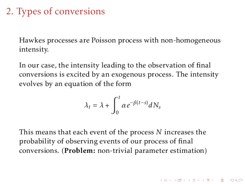
14. 2. Types of conversions Hawkes processes are Poisson process with non-homogeneous intensity. In our case, the intensity leading to the observation of final conversions is excited by an exogenous process. The intensity evolves by an equation of the form λt = λ + t 0 αe−β(t−s)dNs This means that each event of the process N increases the probability of observing events of our process of final conversions. (Problem: non-trivial parameter estimation)
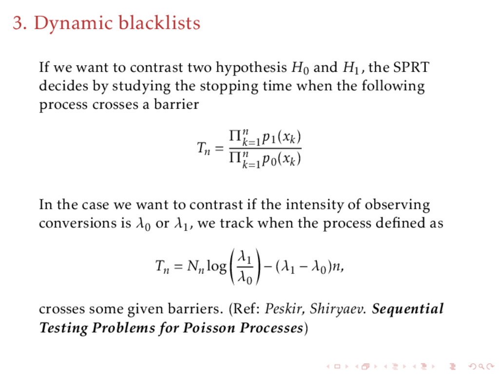
15. 3. Dynamic blacklists As an advertising campaign evolves and we optimize with a finer granularity, we would like to stop spending on domains and placements which are under-performing. Because the campaign evolves and so the data-set is increasing we would like to apply a sequential alternative (instead of classical hypothesis testing or a likelihood-ratio test). Solution: Sequential Probability Ratio Test (SPRT).
16. 3. Dynamic blacklists If we want to contrast two hypothesis H0 and H1, the SPRT decides by studying the stopping time when the following process crosses a barrier Tn = Πn k=1 p1(xk) Πn k=1 p0(xk) In the case we want to contrast if the intensity of observing conversions is λ0 or λ1, we track when the process defined as Tn = Nn log λ1 λ0 − (λ1 − λ0)n, crosses some given barriers. (Ref: Peskir, Shiryaev. Sequential Testing Problems for Poisson Processes)
17. 3. Dynamic blacklists Problem: In practice sequential tests assume we know the parameters λ0 and λ1. In practice at the same time we perform the test, we are estimation λ0 and λ1. The solution of this problem is non-trivial (work in progress: Fernandez-Tapia/Monzani). Strategy vs. Tactics: Allocation, types of conversion and blacklists are ‘Strategic problems’ (focused on CPA). Once we fix a context we need to optimize how to interact with exchanges (i.e. Tactical issues – focus on CPM).
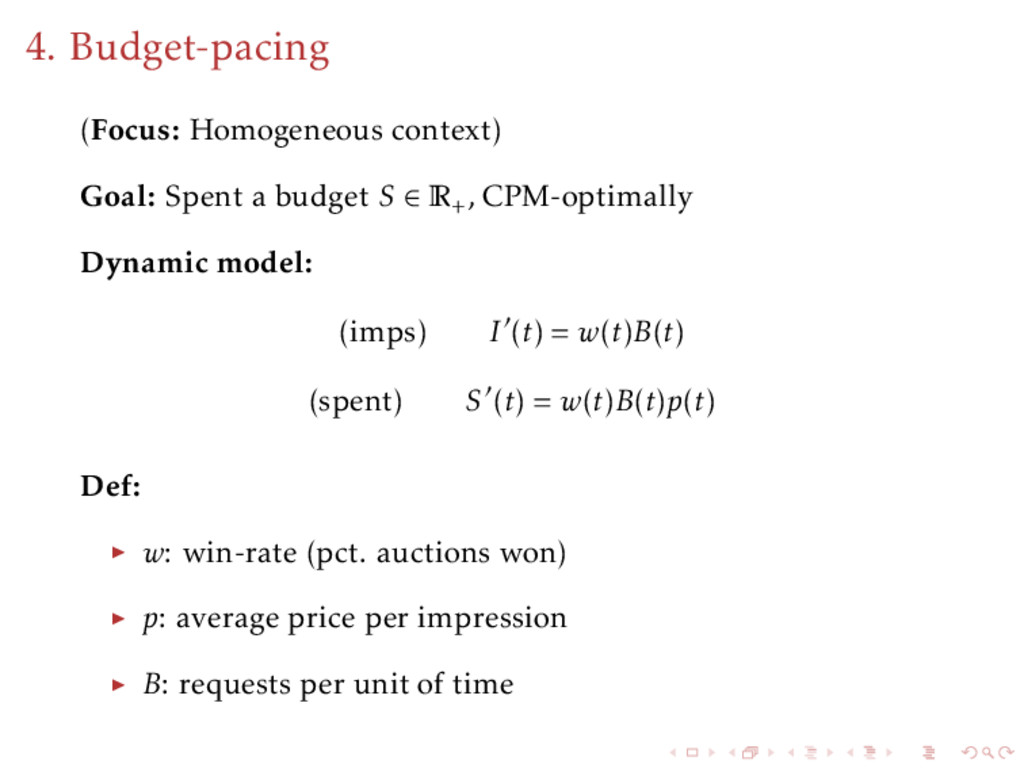
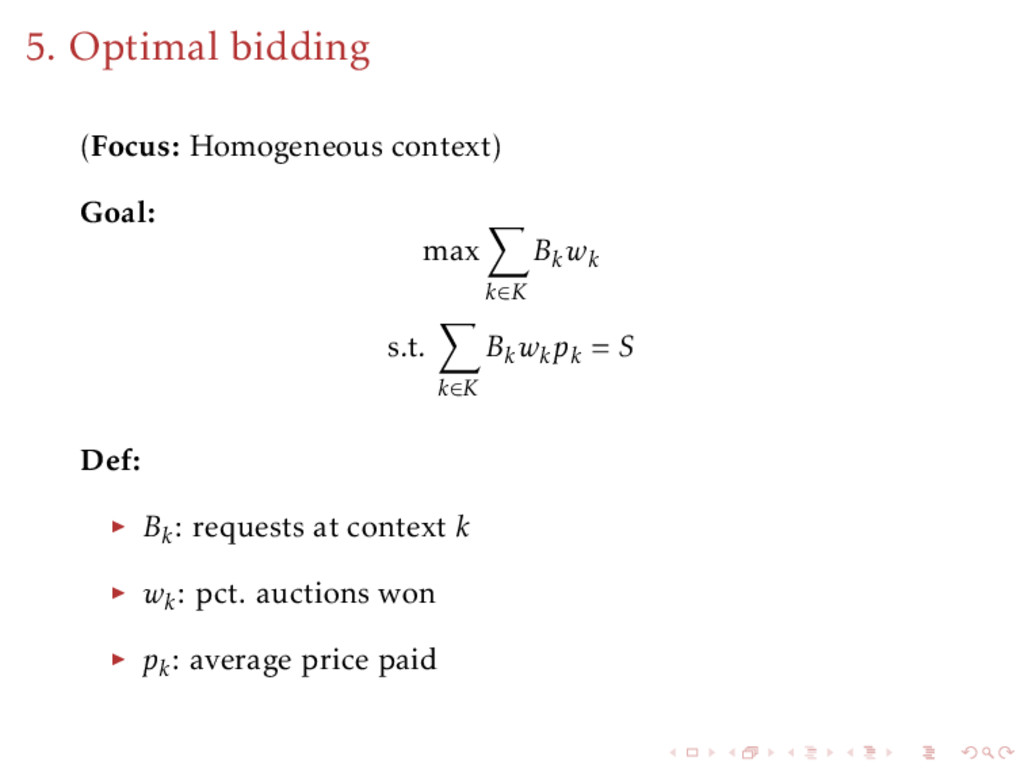
18. 4. Budget-pacing (Focus: Homogeneous context) Goal: Spent a budget S ∈ R+, CPM-optimally Dynamic model: (imps) I (t) = w(t)B(t) (spent) S (t) = w(t)B(t)p(t) Def: w: win-rate (pct. auctions won) p: average price per impression B: requests per unit of time
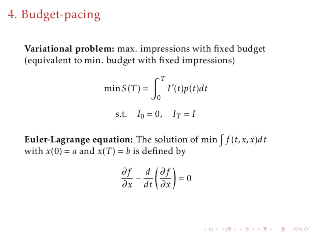
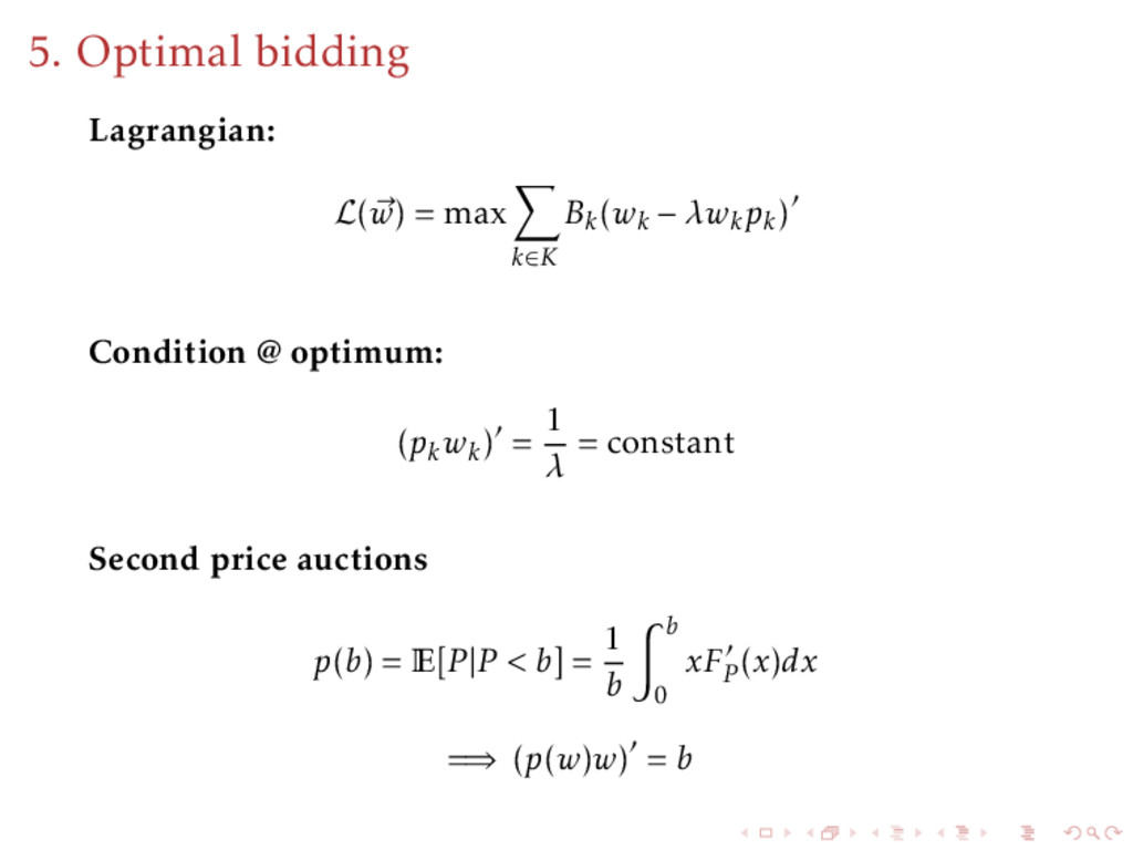
19. 4. Budget-pacing Variational problem: max. impressions with fixed budget (equivalent to min. budget with fixed impressions) minS(T ) = T 0 I (t)p(t)dt s.t. I0 = 0, IT = I Euler-Lagrange equation: The solution of min f (t,x, ˙ x)dt with x(0) = a and x(T ) = b is defined by ∂f ∂x − d dt ∂f ∂ ˙ x = 0
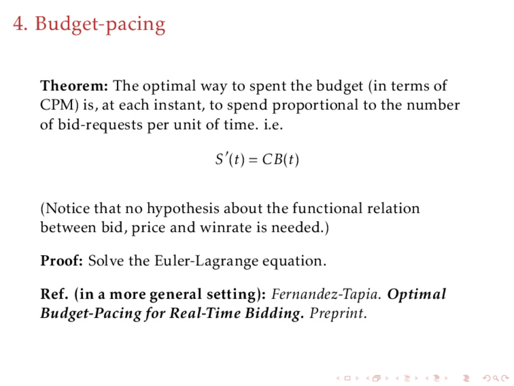
20. 4. Budget-pacing Theorem: The optimal way to spent the budget (in terms of CPM) is, at each instant, to spend proportional to the number of bid-requests per unit of time. i.e. S (t) = CB(t) (Notice that no hypothesis about the functional relation between bid, price and winrate is needed.) Proof: Solve the Euler-Lagrange equation. Ref. (in a more general setting): Fernandez-Tapia. Optimal Budget-Pacing for Real-Time Bidding. Preprint.
21. 5. Optimal bidding (Focus: Homogeneous context) Goal: max k∈K Bkwk s.t. k∈K Bkwkpk = S Def: Bk: requests at context k wk: pct. auctions won pk: average price paid
22. 5. Optimal bidding Lagrangian: L(w) = max k∈K Bk(wk − λwkpk) Condition @ optimum: (pkwk) = 1 λ = constant Second price auctions p(b) = E[P |P < b] = 1 b b 0 xFP (x)dx =⇒ (p(w)w) = b
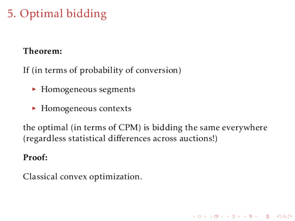
23. 5. Optimal bidding Theorem: If (in terms of probability of conversion) Homogeneous segments Homogeneous contexts the optimal (in terms of CPM) is bidding the same everywhere (regardless statistical differences across auctions!) Proof: Classical convex optimization.
24. Takeaway Viewpoint: top-down/analytical approach Think in terms of homogeneous contexts Classic analysis gives powerful results Strategic issues (allocation, blacklists) Tactical issues (pacing, bidding)
25. References Fernandez-Tapia, J. (2015). Optimal Budget-Pacing for Real-Time Bidding. Available at SSRN 2576212. Fernandez-Tapia, J., & Monzani, C. (2015). Stochastic Multi-Armed Bandit Algorithm for Optimal Budget Allocation in Programmatic Advertising. Available at SSRN 2600473. Narendra, K. S., & Thathachar, M. A. (2012). Learning automata: an introduction. Courier Corporation. Lamberton, D., Pag` es, G., & Tarr` es, P. (2004). When can the two-armed bandit algorithm be trusted?. Annals of Applied Probability, 1424-1454. Peskir, G., & Shiryaev, A. N. (2000). Sequential testing problems for Poisson processes. Annals of Statistics, 837-859.