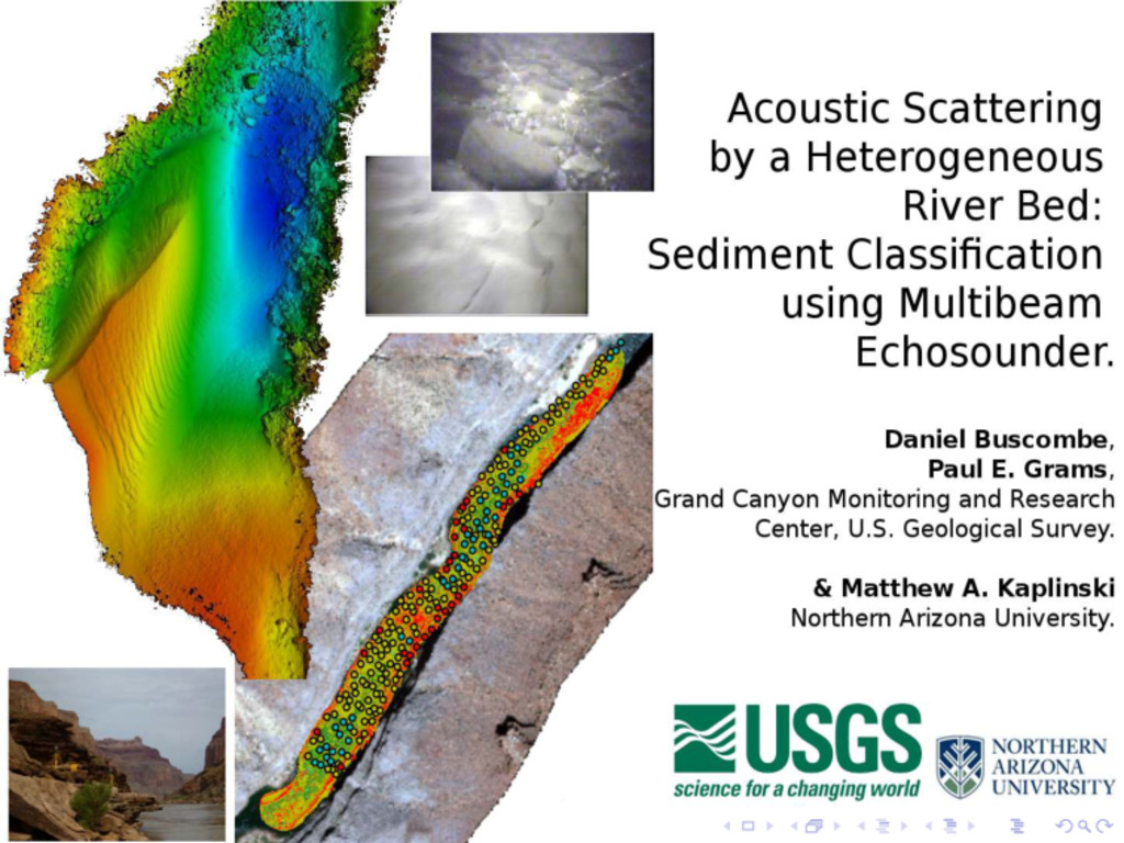
Acoustic Scattering by an Heterogeneous River Bed: Relationship to Bathymetry and Implications for Sediment Classification using Multibeam Echosounder Data
American Geophysical Union Fall Meeting, San Francisco, Dec 2013
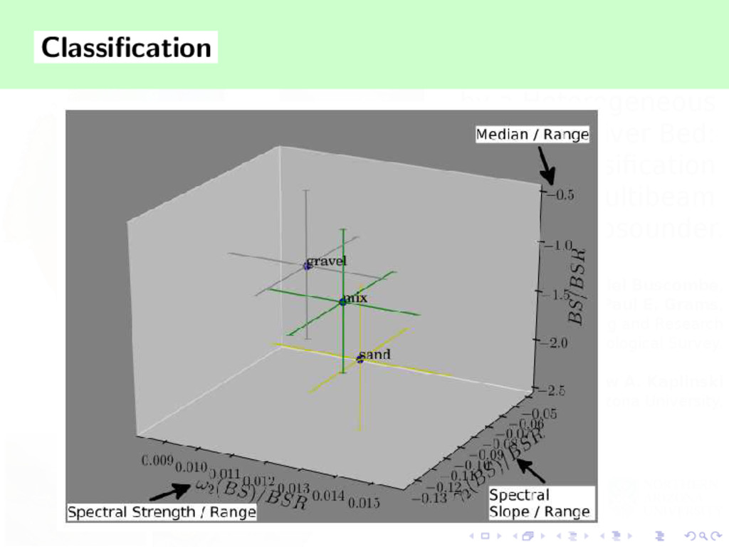
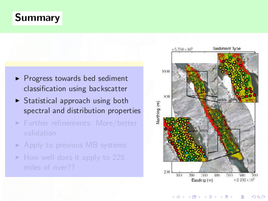
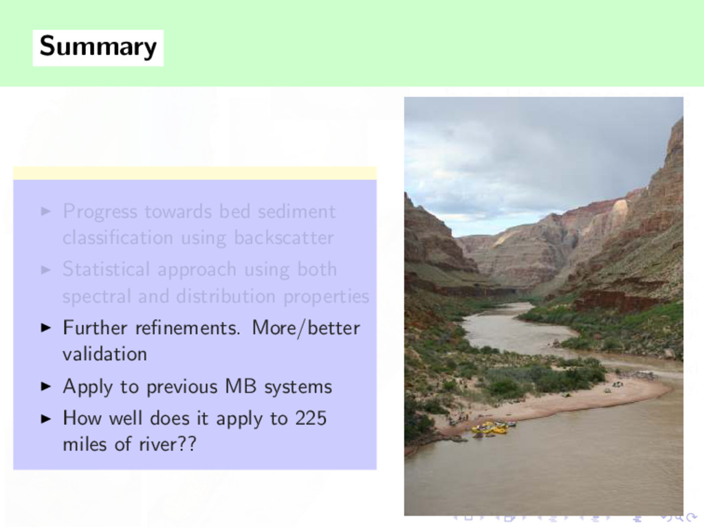
Statistical approach using both spectral and distribution properties ◮ Further refinements. More/better validation ◮ Apply to previous MB systems ◮ How well does it apply to 225 miles of river??
Statistical approach using both spectral and distribution properties ◮ Further refinements. More/better validation ◮ Apply to previous MB systems ◮ How well does it apply to 225 miles of river??
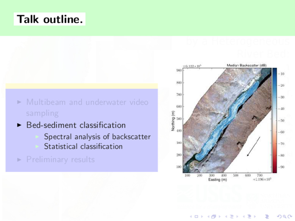
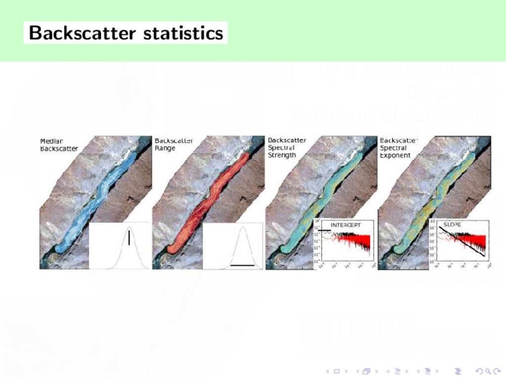
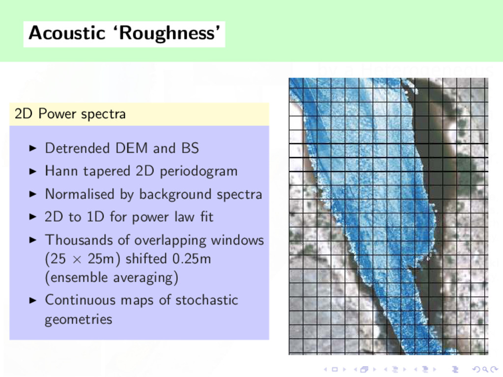
◮ Hann tapered 2D periodogram ◮ Normalised by background spectra ◮ 2D to 1D for power law fit ◮ Thousands of overlapping windows (25 × 25m) shifted 0.25m (ensemble averaging) ◮ Continuous maps of stochastic geometries
Scientific user community ◮ Control and reproducibility Caress and Chayes. Proceedings of the IEEE Oceans 95 Conference, 1995. Caress and Chayes. Marine Geophysical Research, 2006.
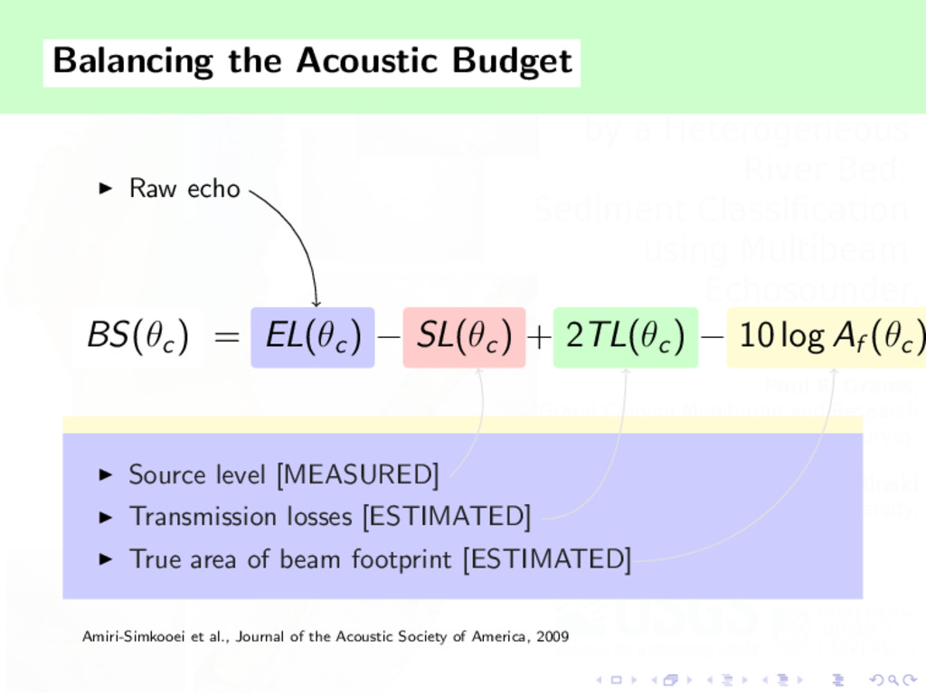
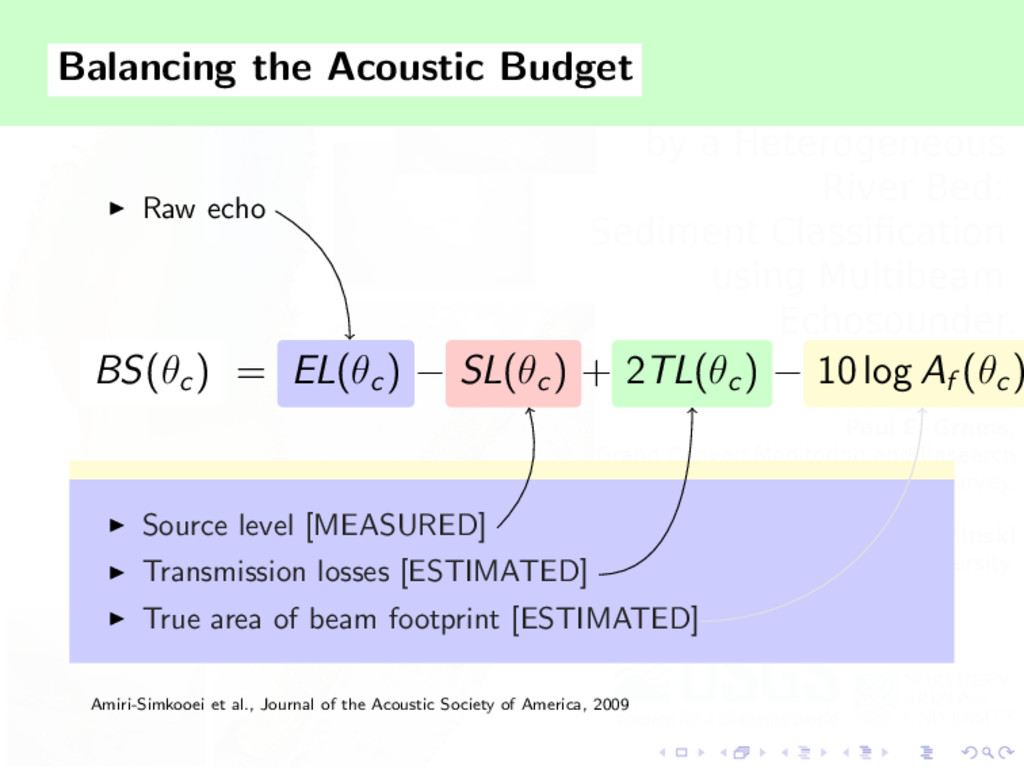
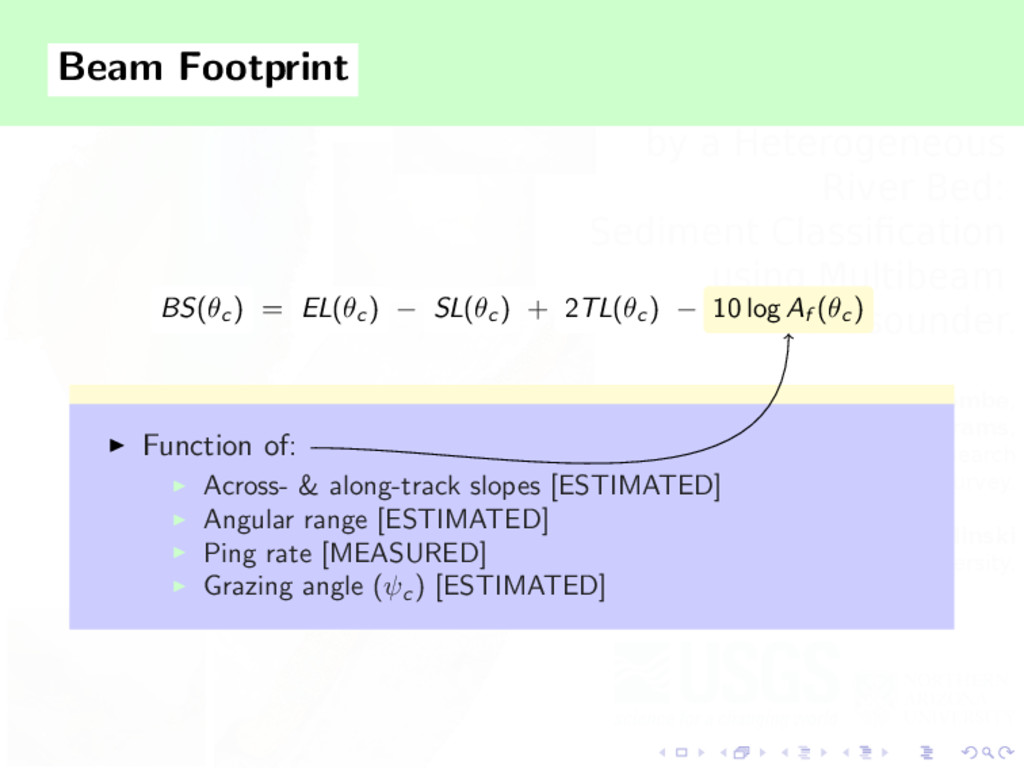
EL(θc ) − SL(θc ) + 2TL(θc ) − 10 log Af (θc ) ◮ Source level [MEASURED] ◮ Transmission losses [ESTIMATED] ◮ True area of beam footprint [ESTIMATED] Amiri-Simkooei et al., Journal of the Acoustic Society of America, 2009
EL(θc ) − SL(θc ) + 2TL(θc ) − 10 log Af (θc ) ◮ Source level [MEASURED] ◮ Transmission losses [ESTIMATED] ◮ True area of beam footprint [ESTIMATED] Amiri-Simkooei et al., Journal of the Acoustic Society of America, 2009
EL(θc ) − SL(θc ) + 2TL(θc ) − 10 log Af (θc ) ◮ Source level [MEASURED] ◮ Transmission losses [ESTIMATED] ◮ True area of beam footprint [ESTIMATED] Amiri-Simkooei et al., Journal of the Acoustic Society of America, 2009
EL(θc ) − SL(θc ) + 2TL(θc ) − 10 log Af (θc ) ◮ Source level [MEASURED] ◮ Transmission losses [ESTIMATED] ◮ True area of beam footprint [ESTIMATED] Amiri-Simkooei et al., Journal of the Acoustic Society of America, 2009
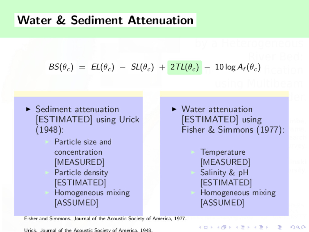
SL(θc ) + 2TL(θc ) − 10 log Af (θc ) ◮ Sediment attenuation [ESTIMATED] using Urick (1948): ◮ Particle size and concentration [MEASURED] ◮ Particle density [ESTIMATED] ◮ Homogeneous mixing [ASSUMED] ◮ Water attenuation [ESTIMATED] using Fisher & Simmons (1977): ◮ Temperature [MEASURED] ◮ Salinity & pH [ESTIMATED] ◮ Homogeneous mixing [ASSUMED] Fisher and Simmons. Journal of the Acoustic Society of America, 1977. Urick. Journal of the Acoustic Society of America, 1948.