VexCL at PECOS, University of Texas, 2013

VexCL - a Vector Expression Template Library for OpenCL

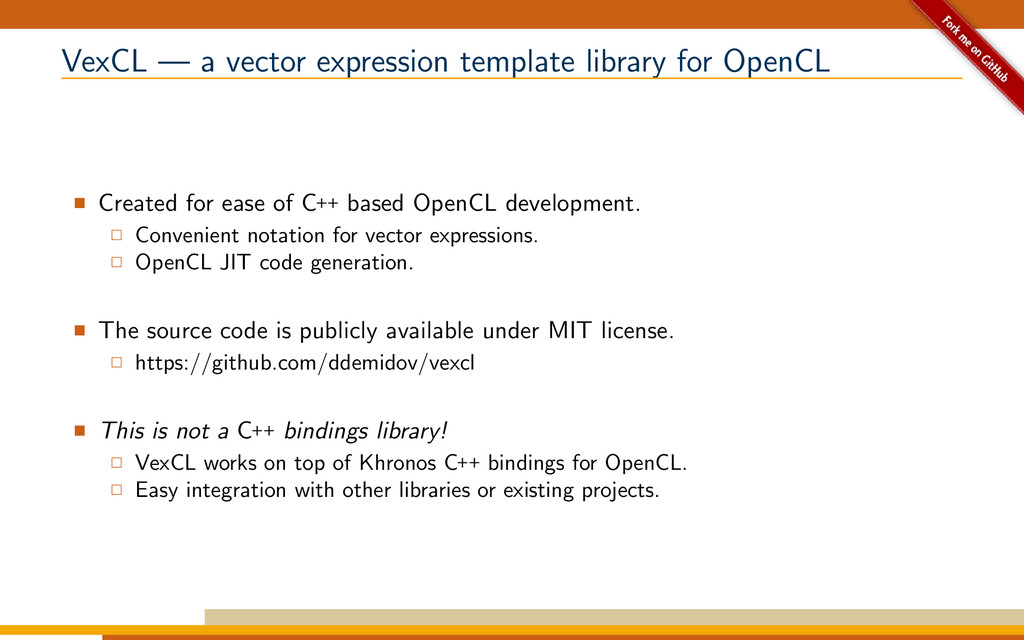
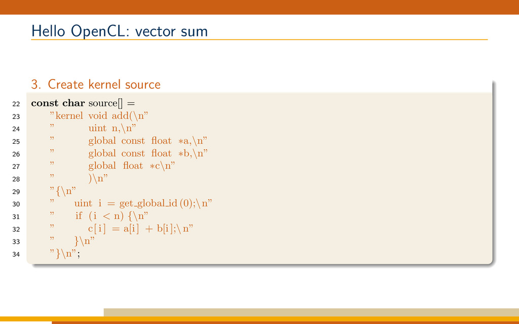
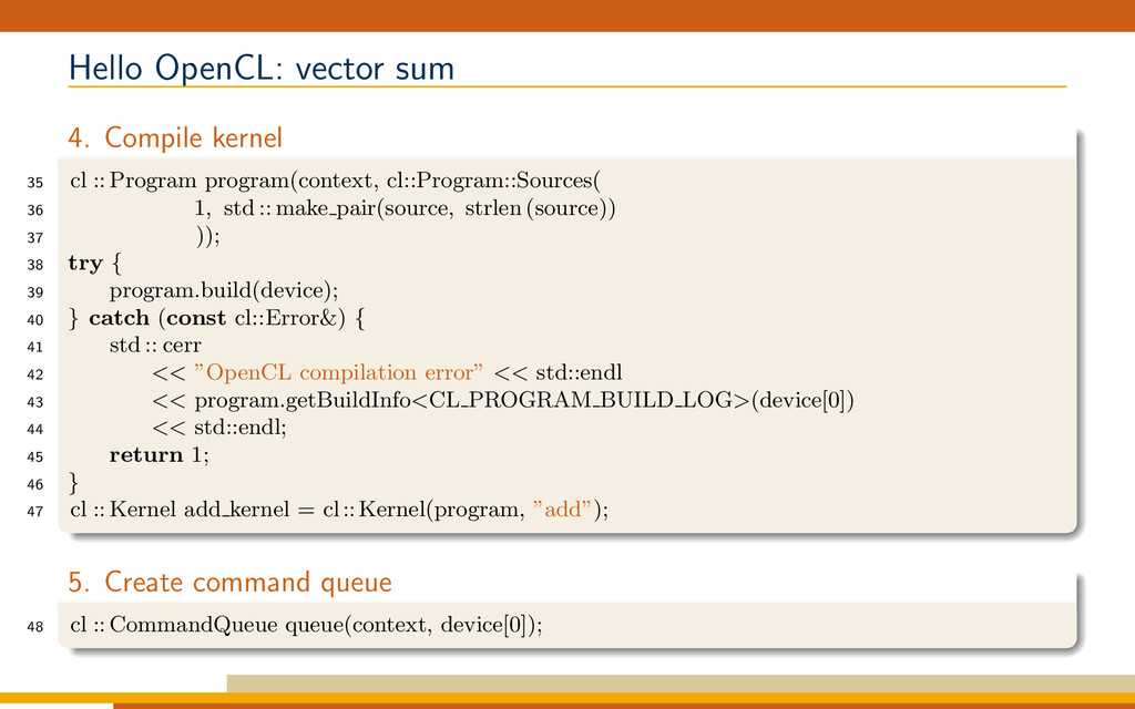
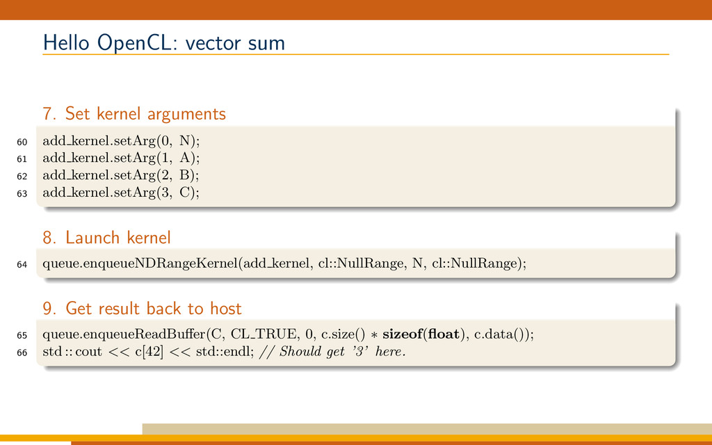
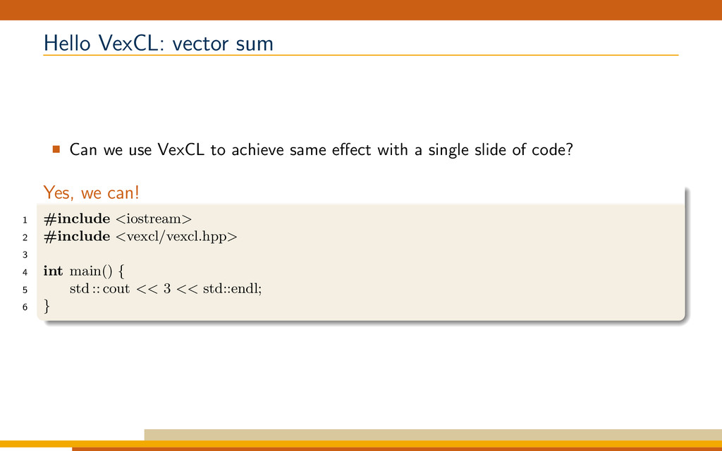
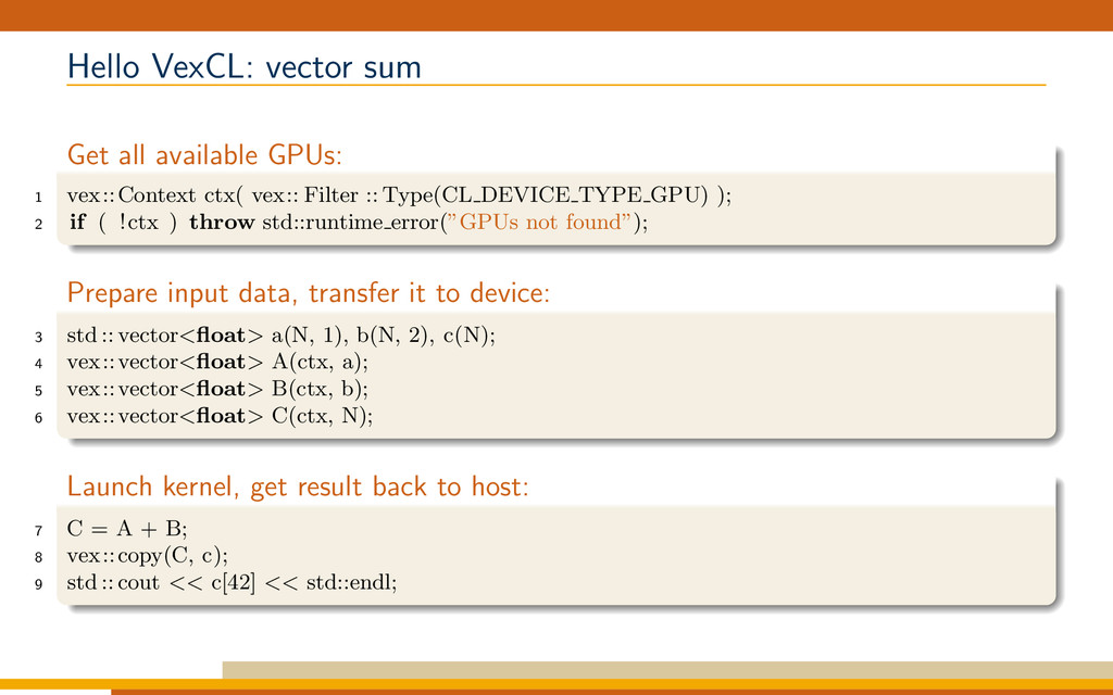
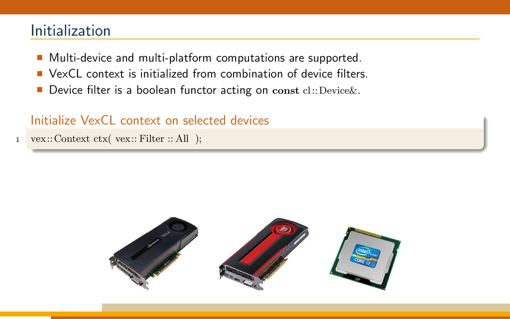
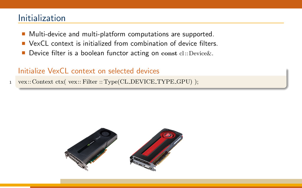
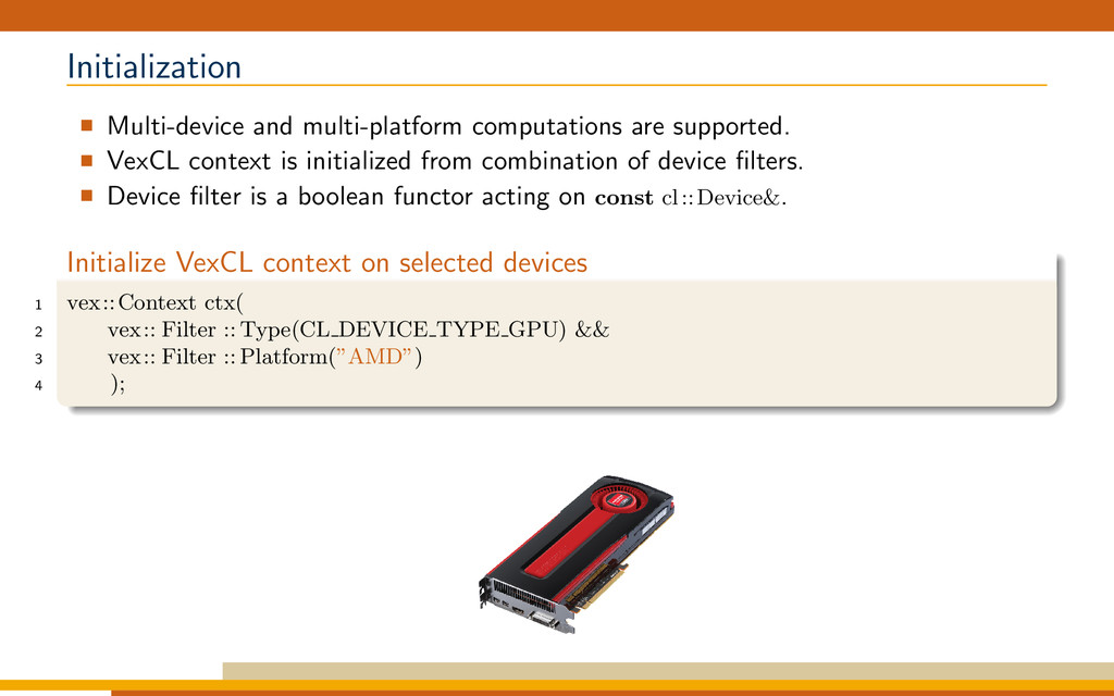
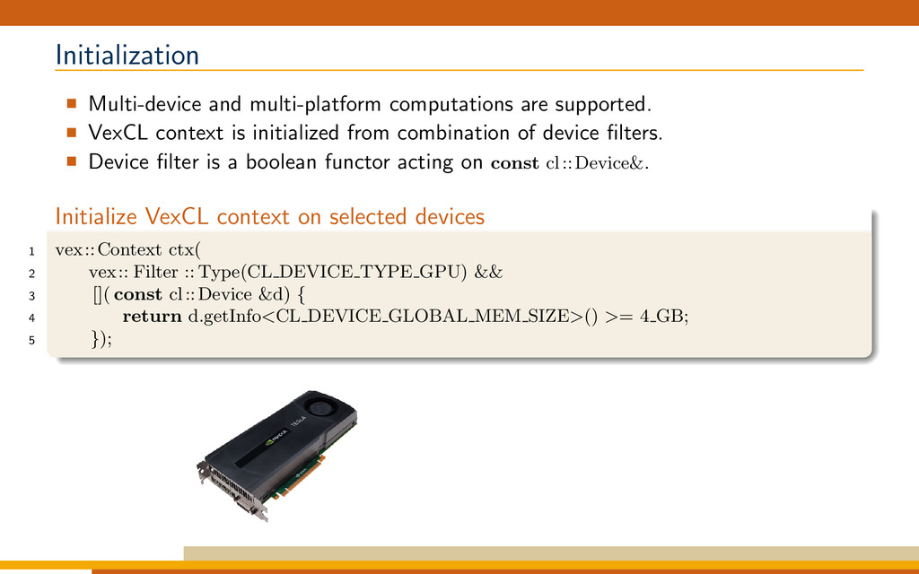
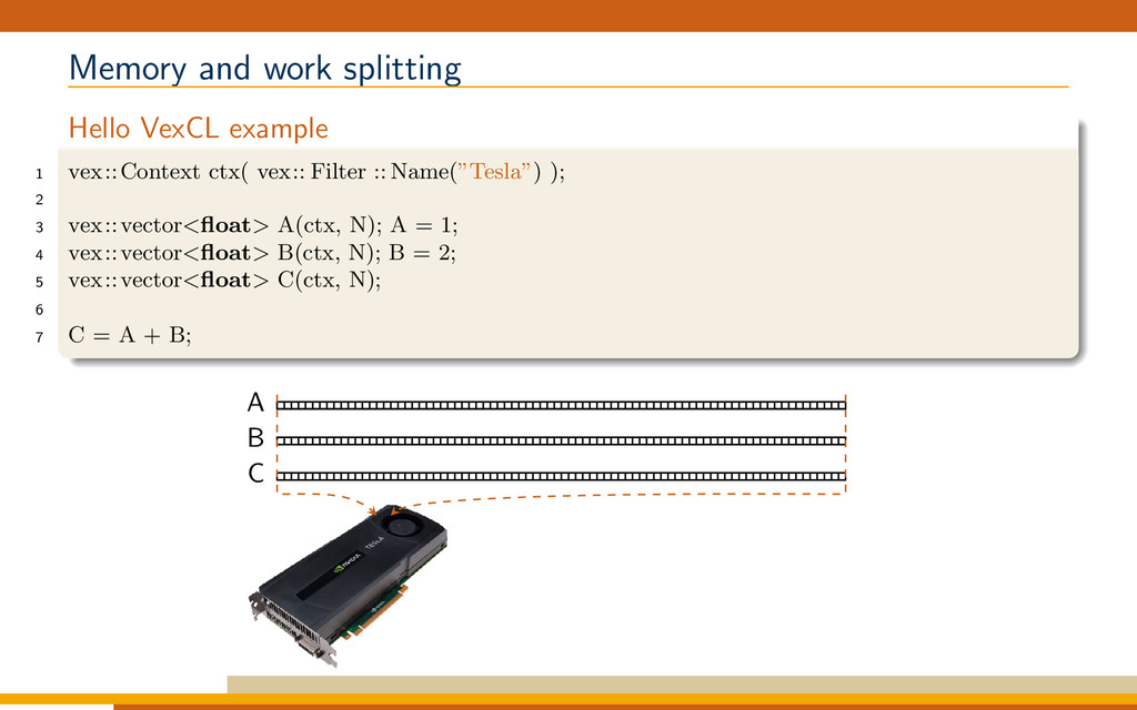
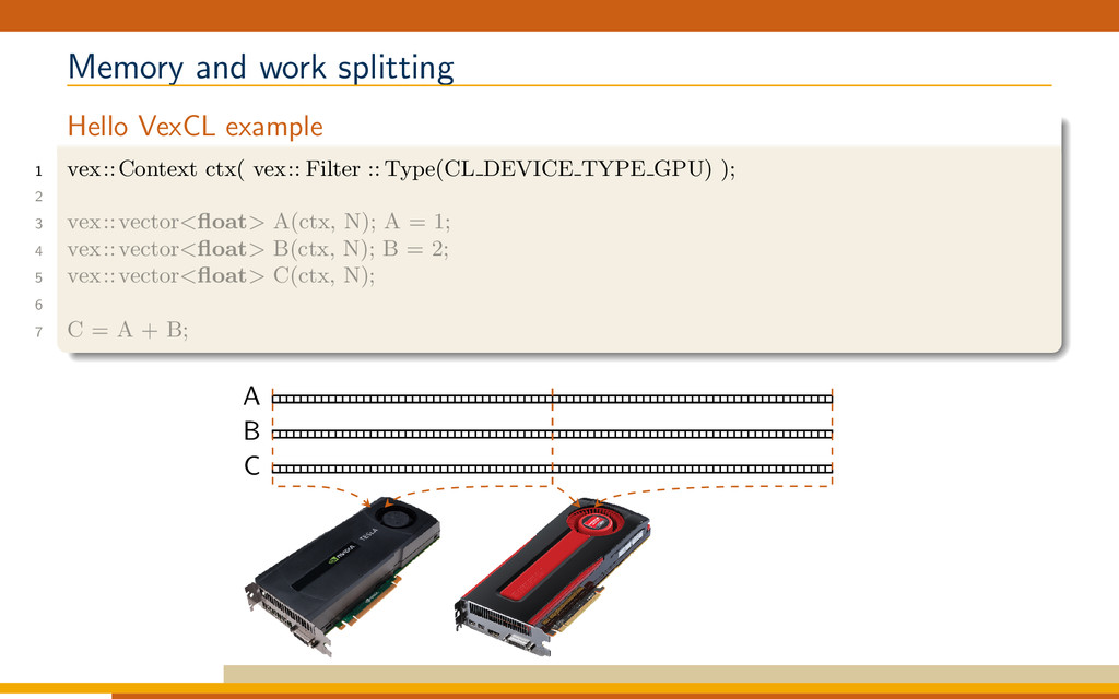
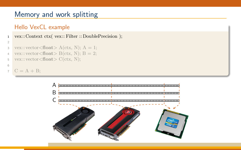
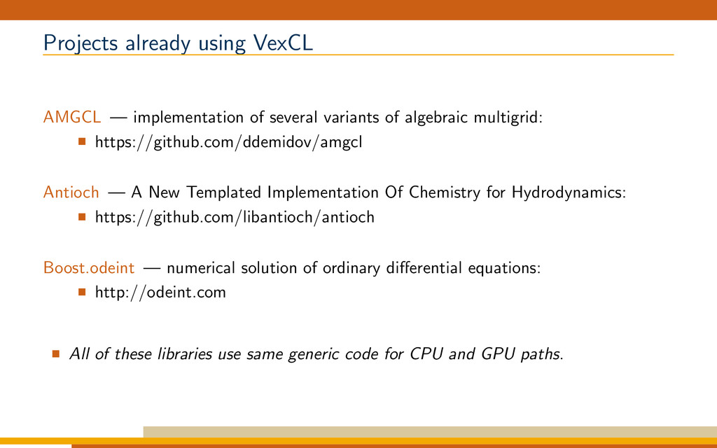
VexCL (https://github.com/ddemidov/vexcl) is a modern C++ library created for ease of OpenCL development with C++. VexCL strives to reduce the amount of boilerplate code needed to develop OpenCL applications. The library provides a convenient and intuitive notation for vector arithmetic, reduction, sparse matrix-vector multiplication, etc. Multidevice and multiplatform computations are supported.

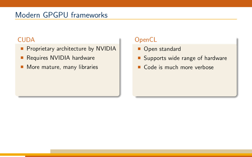
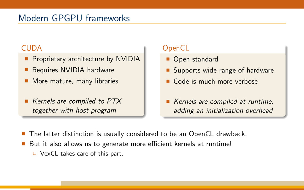
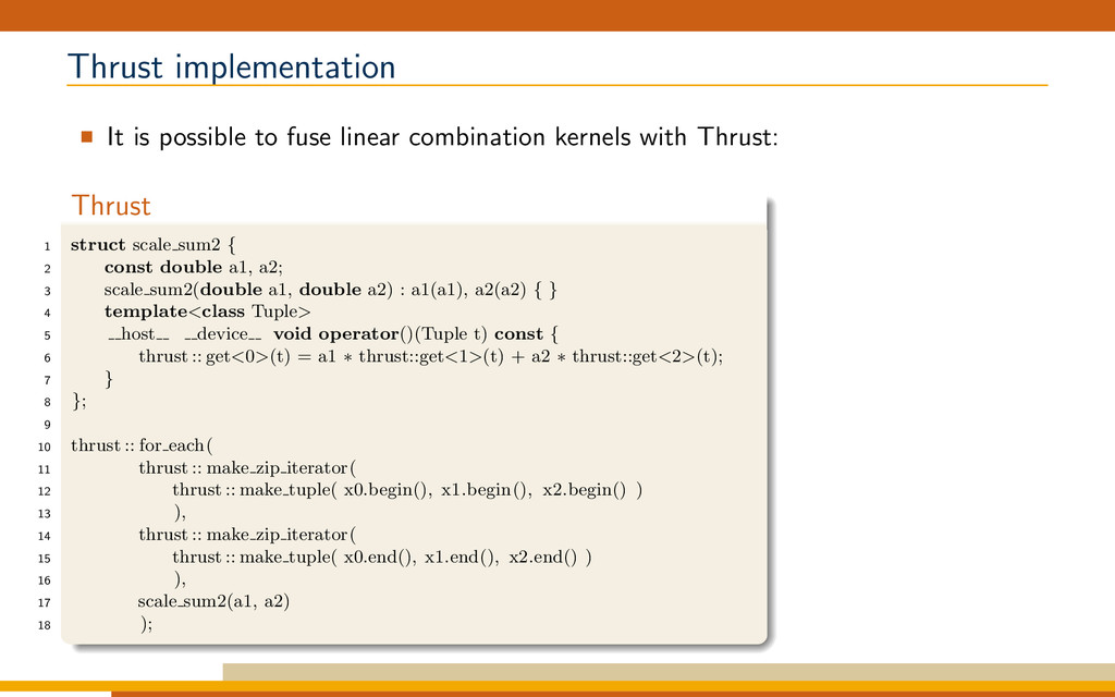
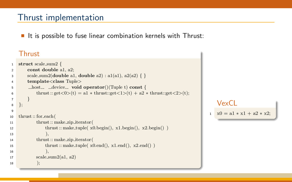
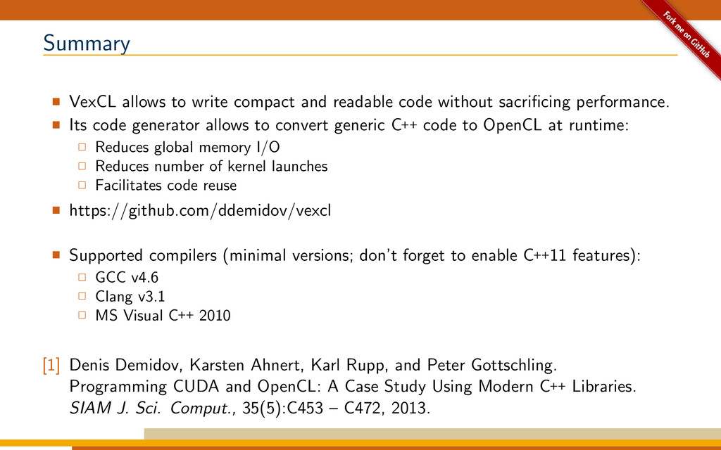
One of the major differences between NVIDIA's CUDA and OpenCL lies in their handling of compute kernels compilation. In NVIDIA’s framework the compute kernels are compiled to PTX code together with the host program. PTX is a pseudo-assembler language which is compiled at runtime for the specific NVIDIA device the kernel is launched on. Since PTX is already very low-level, this just-in-time kernel compilation has low overhead. In OpenCL the compute kernels are compiled at runtime from higher-level C-like sources, adding an overhead which is particularly noticeable for smaller sized problems. At the same time this allows to generate better optimized OpenCL kernels for the problem at hand. The VexCL library exploits this possibility through its JIT code generation facility. It is able to convert generic C++ code to OpenCL at runtime, thus reducing global memory usage and bandwidth. This talk is an introduction to the VexCL interface.

Transcript

1. VexCL — a Vector Expression Template Library for OpenCL
   Denis Demidov
   Supercomputer Center of Russian Academy of Sciences
   Kazan Federal University
   October 2013, Austin, Texas
   

   View Slide

2. Modern GPGPU frameworks
   CUDA
   Proprietary architecture by NVIDIA
   Requires NVIDIA hardware
   More mature, many libraries
   OpenCL
   Open standard
   Supports wide range of hardware
   Code is much more verbose
   

   View Slide

3. Modern GPGPU frameworks
   CUDA
   Proprietary architecture by NVIDIA
   Requires NVIDIA hardware
   More mature, many libraries
   Kernels are compiled to PTX
   together with host program
   OpenCL
   Open standard
   Supports wide range of hardware
   Code is much more verbose
   Kernels are compiled at runtime,
   adding an initialization overhead
   The latter distinction is usually considered to be an OpenCL drawback.
   But it also allows us to generate more efficient kernels at runtime!
   VexCL takes care of this part.
   

   View Slide

4. VexCL — a vector expression template library for OpenCL
   Created for ease of C++ based OpenCL development.
   Convenient notation for vector expressions.
   OpenCL JIT code generation.
   The source code is publicly available under MIT license.
   https://github.com/ddemidov/vexcl
   This is not a C++ bindings library!
   VexCL works on top of Khronos C++ bindings for OpenCL.
   Easy integration with other libraries or existing projects.
   

   View Slide

5. 1 Motivating example
   2 Interface
   3 Is it any good?
   4 Summary
   

   View Slide

6. Hello OpenCL: vector sum
   Compute sum of two vectors in parallel
   A, B, and C are large vectors.
   Compute C = A + B.
   Overview of OpenCL solution:
   1 Initialize OpenCL context on supported device.
   2 Allocate memory on the device.
   3 Transfer input data to device.
   4 Run your computations on the device.
   5 Get the results from the device.
   

   View Slide

7. Hello OpenCL: vector sum
   1. Query platforms
   1 std :: vector platform;
   2 cl :: Platform::get(&platform);
   3
   4 if ( platform.empty() )
   5 throw std::runtime error(”OpenCL platforms not found.”);
   

   View Slide

8. Hello OpenCL: vector sum
   2. Get first available GPU device
   6 cl :: Context context;
   7 std :: vector device;
   8 for(auto p = platform.begin(); device.empty() && p != platform.end(); p++) {
   9 std :: vector dev;
   10 try {
   11 p−>getDevices(CL DEVICE TYPE GPU, &dev);
   12 for(auto d = dev.begin(); device.empty() && d != dev.end(); d++) {
   13 if (!d−>getInfo()) continue;
   14 device.push back(∗d);
   15 context = cl :: Context(device);
   16 }
   17 } catch(...) {
   18 device. clear ();
   19 }
   20 }
   21 if (device.empty()) throw std::runtime error(”GPUs not found”);
   

   View Slide

9. Hello OpenCL: vector sum
   3. Create kernel source
   22 const char source[] =
   23 ”kernel void add(\n”
   24 ” uint n,\n”
   25 ” global const float ∗a,\n”
   26 ” global const float ∗b,\n”
   27 ” global float ∗c\n”
   28 ” )\n”
   29 ”{\n”
   30 ” uint i = get global id (0);\n”
   31 ” if (i < n) {\n”
   32 ” c[ i ] = a[i] + b[i ];\ n”
   33 ” }\n”
   34 ”}\n”;
   

   View Slide

10. Hello OpenCL: vector sum
    4. Compile kernel
    35 cl :: Program program(context, cl::Program::Sources(
    36 1, std :: make pair(source, strlen (source))
    37 ));
    38 try {
    39 program.build(device);
    40 } catch (const cl::Error&) {
    41 std :: cerr
    42 << ”OpenCL compilation error” << std::endl
    43 << program.getBuildInfo(device[0])
    44 << std::endl;
    45 return 1;
    46 }
    47 cl :: Kernel add kernel = cl::Kernel(program, ”add”);
    5. Create command queue
    48 cl :: CommandQueue queue(context, device[0]);
    

    View Slide

11. Hello OpenCL: vector sum
    6. Prepare input data, transfer it to device
    49 const size t N = 1 << 20;
    50 std :: vector<float> a(N, 1), b(N, 2), c(N);
    51
    52 cl :: Buffer A(context, CL MEM READ ONLY | CL MEM COPY HOST PTR,
    53 a. size () ∗ sizeof(float), a.data());
    54
    55 cl :: Buffer B(context, CL MEM READ ONLY | CL MEM COPY HOST PTR,
    56 b. size () ∗ sizeof(float), b.data());
    57
    58 cl :: Buffer C(context, CL MEM READ WRITE,
    59 c. size () ∗ sizeof(float ));
    

    View Slide

12. Hello OpenCL: vector sum
    7. Set kernel arguments
    60 add kernel.setArg(0, N);
    61 add kernel.setArg(1, A);
    62 add kernel.setArg(2, B);
    63 add kernel.setArg(3, C);
    8. Launch kernel
    64 queue.enqueueNDRangeKernel(add kernel, cl::NullRange, N, cl::NullRange);
    9. Get result back to host
    65 queue.enqueueReadBuffer(C, CL TRUE, 0, c.size() ∗ sizeof(float), c.data());
    66 std :: cout << c[42] << std::endl; // Should get ’3’ here.
    

    View Slide

13. Hello VexCL: vector sum
    Can we use VexCL to achieve same effect with a single slide of code?
    

    View Slide

14. Hello VexCL: vector sum
    Can we use VexCL to achieve same effect with a single slide of code?
    Yes, we can!
    1 #include
    2 #include
    3
    4 int main() {
    5 std :: cout << 3 << std::endl;
    6 }
    

    View Slide

15. Hello VexCL: vector sum
    Get all available GPUs:
    1 vex::Context ctx( vex:: Filter :: Type(CL DEVICE TYPE GPU) );
    2 if ( !ctx ) throw std::runtime error(”GPUs not found”);
    Prepare input data, transfer it to device:
    3 std :: vector<float> a(N, 1), b(N, 2), c(N);
    4 vex::vector<float> A(ctx, a);
    5 vex::vector<float> B(ctx, b);
    6 vex::vector<float> C(ctx, N);
    Launch kernel, get result back to host:
    7 C = A + B;
    8 vex::copy(C, c);
    9 std :: cout << c[42] << std::endl;
    

    View Slide

16. 1 Motivating example
    2 Interface
    3 Is it any good?
    4 Summary
    

    View Slide

17. Initialization
    Multi-device and multi-platform computations are supported.
    VexCL context is initialized from combination of device filters.
    Device filter is a boolean functor acting on const cl::Device&.
    Initialize VexCL context on selected devices
    1 vex::Context ctx( vex:: Filter :: All );
    

    View Slide

18. Initialization
    Multi-device and multi-platform computations are supported.
    VexCL context is initialized from combination of device filters.
    Device filter is a boolean functor acting on const cl::Device&.
    Initialize VexCL context on selected devices
    1 vex::Context ctx( vex:: Filter :: Type(CL DEVICE TYPE GPU) );
    

    View Slide

19. Initialization
    Multi-device and multi-platform computations are supported.
    VexCL context is initialized from combination of device filters.
    Device filter is a boolean functor acting on const cl::Device&.
    Initialize VexCL context on selected devices
    1 vex::Context ctx(
    2 vex:: Filter :: Type(CL DEVICE TYPE GPU) &&
    3 vex:: Filter :: Platform(”AMD”)
    4 );
    

    View Slide

20. Initialization
    Multi-device and multi-platform computations are supported.
    VexCL context is initialized from combination of device filters.
    Device filter is a boolean functor acting on const cl::Device&.
    Initialize VexCL context on selected devices
    1 vex::Context ctx(
    2 vex:: Filter :: Type(CL DEVICE TYPE GPU) &&
    3 []( const cl::Device &d) {
    4 return d.getInfo() >= 4 GB;
    5 });
    

    View Slide

21. Exclusive device access
    vex:: Filter :: Exclusive() wraps normal filters to allow exclusive access to devices.
    Useful for MPI jobs.
    An alternative to NVIDIA’s exclusive compute mode for other vendors hardware.
    Based on Boost.Interprocess file locks in temp directory.
    Use VEXCL LOCK DIR environment variable to override default behavior.
    1 vex::Context ctx( vex:: Filter :: Exclusive (
    2 vex:: Filter :: Env && vex::Filter::Count(1)
    3 ) );
    Only works between programs that actually use the filter.
    

    View Slide

22. Memory and work splitting
    Hello VexCL example
    1 vex::Context ctx( vex:: Filter :: Name(”Tesla”) );
    2
    3 vex::vector<float> A(ctx, N); A = 1;
    4 vex::vector<float> B(ctx, N); B = 2;
    5 vex::vector<float> C(ctx, N);
    6
    7 C = A + B;
    A
    B
    C
    

    View Slide

23. Memory and work splitting
    Hello VexCL example
    1 vex::Context ctx( vex:: Filter :: Type(CL DEVICE TYPE GPU) );
    2
    3 vex::vector<float> A(ctx, N); A = 1;
    4 vex::vector<float> B(ctx, N); B = 2;
    5 vex::vector<float> C(ctx, N);
    6
    7 C = A + B;
    A
    B
    C
    

    View Slide

24. Memory and work splitting
    Hello VexCL example
    1 vex::Context ctx( vex:: Filter :: DoublePrecision );
    2
    3 vex::vector<float> A(ctx, N); A = 1;
    4 vex::vector<float> B(ctx, N); B = 2;
    5 vex::vector<float> C(ctx, N);
    6
    7 C = A + B;
    A
    B
    C
    

    View Slide

25. Copies between host and device memory
    1 vex::vector d(ctx, n);
    2 std :: vector h(n);
    3 double a[100];
    Simple copies
    1 vex::copy(d, h);
    2 vex::copy(h, d);
    

    View Slide

26. Copies between host and device memory
    1 vex::vector d(ctx, n);
    2 std :: vector h(n);
    3 double a[100];
    Simple copies
    1 vex::copy(d, h);
    2 vex::copy(h, d);
    STL-like range copies
    1 vex::copy(d.begin(), d.end(), h.begin());
    2 vex::copy(d.begin(), d.begin() + 100, a);
    

    View Slide

27. Copies between host and device memory
    1 vex::vector d(ctx, n);
    2 std :: vector h(n);
    3 double a[100];
    Simple copies
    1 vex::copy(d, h);
    2 vex::copy(h, d);
    STL-like range copies
    1 vex::copy(d.begin(), d.end(), h.begin());
    2 vex::copy(d.begin(), d.begin() + 100, a);
    Map OpenCL buffer to host pointer
    1 auto p = d.map(devnum);
    2 std :: sort(&p[0], &p[d.part size(devnum)]);
    

    View Slide

28. Copies between host and device memory
    1 vex::vector d(ctx, n);
    2 std :: vector h(n);
    3 double a[100];
    Simple copies
    1 vex::copy(d, h);
    2 vex::copy(h, d);
    STL-like range copies
    1 vex::copy(d.begin(), d.end(), h.begin());
    2 vex::copy(d.begin(), d.begin() + 100, a);
    Map OpenCL buffer to host pointer
    1 auto p = d.map(devnum);
    2 std :: sort(&p[0], &p[d.part size(devnum)]);
    Inspect or set single element (slow)
    1 double v = d[42];
    2 d[0] = 0;
    

    View Slide

29. What vector expressions are supported?
    All vectors in an expression have to be compatible:
    Have same size
    Located on same devices
    What may be used:
    Vectors and scalars
    Arithmetic, logical operators
    Built-in OpenCL functions
    User-defined functions
    Random number generators
    Slicing and permutations
    Reduction (sum, min, max)
    Stencil operations
    Sparse matrix – vector products
    Fast Fourier Transform
    1 vex::vector x(ctx, n), y(ctx, n);
    2
    3 x = 2 ∗ M PI ∗ vex::element index() / n;
    4 y = pow(sin(x), 2.0) + pow(cos(x), 2.0);
    

    View Slide

30. Builtin operations and functions
    This expression:
    1 x = 2 ∗ y − sin(z);
    Define VEXCL SHOW KERNELS to see the
    generated code.
    . . . results in this kernel:
    1 kernel void vexcl vector kernel(
    2 ulong n,
    3 global double ∗ prm 1,
    4 int prm 2,
    5 global double ∗ prm 3,
    6 global double ∗ prm 4
    7 )
    8 {
    9 for(size t idx = get global id(0); idx < n; idx += get global size(0)) {
    10 prm 1[idx] = ( ( prm 2 ∗ prm 3[idx] ) − sin( prm 4[idx] ) );
    11 }
    12 }
    −
    ∗ sin
    2 y z
    

    View Slide

31. Constants
    Macro VEX CONSTANT allows to define literal constants
    1 VEX CONSTANT(two, 2);
    2 x = two() ∗ y − sin(z);
    1 kernel void vexcl vector kernel(
    2 ulong n,
    3 global double ∗ prm 1,
    4 global double ∗ prm 3,
    5 global double ∗ prm 4
    6 )
    7 {
    8 for(size t idx = get global id(0); idx < n; idx += get global size(0)) {
    9 prm 1[idx] = ( ( ( 2 ) ∗ prm 3[idx] ) − sin( prm 4[idx] ) );
    10 }
    11 }
    Some predefined math constants are available (wrappers to boost::math::constants):
    vex::constants :: pi(), vex::constants :: root two(), etc.
    

    View Slide

32. Element indices
    vex::element index(size t offset = 0) returns index of an element inside a vector.
    The numbering starts with offset and is continuous across devices.
    Linear function:
    1 vex::vector X(ctx, N);
    2 double x0 = 0, dx = 1e−3;
    3 X = x0 + dx ∗ vex::element index();
    Single period of sine function:
    1 X = sin(vex::constants :: two pi() ∗ vex::element index() / N);
    

    View Slide

33. User-defined functions
    Users may define functions to be used in vector expressions.
    There are two options for doing this:
    Provide function body in a string.
    Provide generic C++ functor.
    Once defined, user functions are used in the same way as builtin functions.
    

    View Slide

34. 1. Provide function body in a string
    Choose function name
    Specify function signature
    Provide function body
    Defining a function:
    1 VEX FUNCTION( sqr, double(double, double), ”return prm1 ∗ prm1 + prm2 ∗ prm2;” );
    Using a function:
    1 Z = sqrt( sqr(X, Y) );
    

    View Slide

35. 2. Provide generic functor
    Functor definition:
    1 struct sqr functor {
    2 template
    3 T operator()(const T &x, const T &y) const {
    4 return x ∗ x + y ∗ y;
    5 }
    6 };
    

    View Slide

36. 2. Provide generic functor
    Functor definition:
    1 struct sqr functor {
    2 template
    3 T operator()(const T &x, const T &y) const {
    4 return x ∗ x + y ∗ y;
    5 }
    6 };
    Generate VexCL function:
    1 using vex::generator::make function;
    2 auto sqr = make function( sqr functor() );
    

    View Slide

37. 2. Provide generic functor
    Functor definition:
    1 struct sqr functor {
    2 template
    3 T operator()(const T &x, const T &y) const {
    4 return x ∗ x + y ∗ y;
    5 }
    6 };
    Generate VexCL function:
    1 using vex::generator::make function;
    2 auto sqr = make function( sqr functor() );
    Boost.Phoenix lambdas are generic functors:
    1 using namespace boost::phoenix::arg names;
    2 auto sqr = make function( arg1 ∗ arg1 + arg2 ∗ arg2 );
    

    View Slide

38. User functions are translated to OpenCL functions
    1 Z = sqrt( sqr(X, Y) );
    . . . gets translated to:
    1 double func1(double prm1, double prm2) {
    2 return prm1 ∗ prm1 + prm2 ∗ prm2;
    3 }
    4
    5 kernel void vexcl vector kernel(
    6 ulong n,
    7 global double ∗ prm 1,
    8 global double ∗ prm 2,
    9 global double ∗ prm 3
    10 )
    11 {
    12 for(size t idx = get global id(0); idx < n; idx += get global size(0)) {
    13 prm 1[idx] = sqrt( func1( prm 2[idx], prm 3[idx] ) );
    14 }
    15 }
    sqrt
    sqr
    x y
    

    View Slide

39. Functions may be not only convenient, but also effective
    Same example without using a function:
    1 Z = sqrt( X ∗ X + Y ∗ Y );
    . . . gets translated to:
    1 kernel void vexcl vector kernel(
    2 ulong n,
    3 global double ∗ prm 1,
    4 global double ∗ prm 2,
    5 global double ∗ prm 3,
    6 global double ∗ prm 4,
    7 global double ∗ prm 5
    8 )
    9 {
    10 for(size t idx = get global id(0); idx < n; idx += get global size(0)) {
    11 prm 1[idx] = sqrt( ( ( prm 2[idx] ∗ prm 3[idx] ) + ( prm 4[idx] ∗ prm 5[idx] ) ) );
    12 }
    13 }
    sqrt
    +
    ∗ ∗
    x x y y
    

    View Slide

40. Tagged terminals
    Programmer may help VexCL to recognize same terminals by tagging them:
    Like this:
    1 using vex::tag;
    2 Z = sqrt(tag<1>(X) ∗ tag<1>(X) +
    3 tag<2>(Y) ∗ tag<2>(Y));
    or, equivalently:
    1 auto x = tag<1>(X);
    2 auto y = tag<2>(Y);
    3 Z = sqrt(x ∗ x + y ∗ y);
    1 kernel void vexcl vector kernel(
    2 ulong n,
    3 global double ∗ prm 1,
    4 global double ∗ prm 2,
    5 global double ∗ prm 3
    6 )
    7 {
    8 for(size t idx = get global id(0); idx < n; idx += get global size(0)) {
    9 prm 1[idx] = sqrt( ( ( prm 2[idx] ∗ prm 2[idx] ) + ( prm 3[idx] ∗ prm 3[idx] ) ) );
    10 }
    11 }
    

    View Slide

41. Reusing intermediate results
    Some expressions may have several
    inclusions of the same subexpression:
    1 Z = log(X) ∗ (log(X) + Y);
    log(X) will be computed twice here.
    One could tag X and hope that
    OpenCL compiler is smart enough. . .
    ∗
    +
    log
    log
    x
    x
    y
    

    View Slide

42. Temporaries
    But it is also possible to introduce a temporary variable explicitly:
    1 auto tmp = vex::make temp<1>( log(X) );
    2 Z = tmp ∗ (tmp + Y);
    1 kernel void vexcl vector kernel(
    2 ulong n,
    3 global double ∗ prm 1,
    4 global double ∗ prm 2,
    5 global double ∗ prm 3
    6 )
    7 {
    8 for(size t idx = get global id(0); idx < n; idx += get global size(0)) {
    9 double temp 1 = log( prm 2[idx] );
    10 prm 1[idx] = ( temp 1 ∗ ( temp 1 + prm 3[idx] ) );
    11 }
    12 }
    

    View Slide

43. Permutations (Single-device contexts)
    vex::permutation() function takes arbitrary (integral valued) vector expression and
    returns permutation functor:
    

    View Slide

44. Permutations (Single-device contexts)
    vex::permutation() function takes arbitrary (integral valued) vector expression and
    returns permutation functor:
    Index-based permutation:
    1 vex::vector I(ctx, N);
    2 I = N − 1 − vex::element index();
    3 auto reverse = vex::permutation(I);
    4 y = reverse(x);
    

    View Slide

45. Permutations (Single-device contexts)
    vex::permutation() function takes arbitrary (integral valued) vector expression and
    returns permutation functor:
    Index-based permutation:
    1 vex::vector I(ctx, N);
    2 I = N − 1 − vex::element index();
    3 auto reverse = vex::permutation(I);
    4 y = reverse(x);
    Expression-based permutation:
    1 auto reverse = vex::permutation(N − 1 − vex::element index());
    2 y = reverse(x);
    

    View Slide

46. Permutations (Single-device contexts)
    vex::permutation() function takes arbitrary (integral valued) vector expression and
    returns permutation functor:
    Index-based permutation:
    1 vex::vector I(ctx, N);
    2 I = N − 1 − vex::element index();
    3 auto reverse = vex::permutation(I);
    4 y = reverse(x);
    Expression-based permutation:
    1 auto reverse = vex::permutation(N − 1 − vex::element index());
    2 y = reverse(x);
    Permutations are writable:
    1 reverse(y) = x;
    

    View Slide

47. Slicing (Single-device contexts)
    When working with dense multidimensional matrices, it is general practice to store
    those in continuous arrays.
    An instance of vex:: slicer class allows to access sub-blocks of such matrix.
    n-by-n matrix and a slicer:
    1 vex::vector x(ctx, n ∗ n);
    2 vex:: slicer <2> slice(vex::extents[n][n ]); // Can be used with any vector of appropriate size
    

    View Slide

48. Slicing (Single-device contexts)
    When working with dense multidimensional matrices, it is general practice to store
    those in continuous arrays.
    An instance of vex:: slicer class allows to access sub-blocks of such matrix.
    n-by-n matrix and a slicer:
    1 vex::vector x(ctx, n ∗ n);
    2 vex:: slicer <2> slice(vex::extents[n][n ]); // Can be used with any vector of appropriate size
    Access row or column of the matrix:
    3 using vex:: ;
    4 y = slice [42]( x); // 42nd row
    5 y = slice [ ][42]( x); // 42nd column
    6 slice [ ][10]( x) = y; // Slices are writable
    

    View Slide

49. Slicing (Single-device contexts)
    When working with dense multidimensional matrices, it is general practice to store
    those in continuous arrays.
    An instance of vex:: slicer class allows to access sub-blocks of such matrix.
    n-by-n matrix and a slicer:
    1 vex::vector x(ctx, n ∗ n);
    2 vex:: slicer <2> slice(vex::extents[n][n ]); // Can be used with any vector of appropriate size
    Access row or column of the matrix:
    3 using vex:: ;
    4 y = slice [42]( x); // 42nd row
    5 y = slice [ ][42]( x); // 42nd column
    6 slice [ ][10]( x) = y; // Slices are writable
    Use ranges to select sub-blocks:
    7 using vex::range;
    8 z = slice [range(0, 2, n )][ range(10, 20)](x);
    

    View Slide

50. Reducing slices (Single-device contexts)
    vex::reduce() function takes multidimensional slice of arbitrary expression and
    reduces it along one or more dimensions.
    Supported reduction kinds: SUM, MIN, MAX.
    Row-wise sum:
    1 vex:: slicer <2> s(extents[n][n]);
    2 y = vex::reduce(s[ ], x, 1);
    

    View Slide

51. Reducing slices (Single-device contexts)
    vex::reduce() function takes multidimensional slice of arbitrary expression and
    reduces it along one or more dimensions.
    Supported reduction kinds: SUM, MIN, MAX.
    Row-wise sum:
    1 vex:: slicer <2> s(extents[n][n]);
    2 y = vex::reduce(s[ ], x, 1);
    Column-wise maximum absolute value:
    1 vex:: slicer <2> s(extents[n][n]);
    2 y = vex::reduce(s[ ], fabs(x), 0);
    

    View Slide

52. Reducing slices (Single-device contexts)
    vex::reduce() function takes multidimensional slice of arbitrary expression and
    reduces it along one or more dimensions.
    Supported reduction kinds: SUM, MIN, MAX.
    Row-wise sum:
    1 vex:: slicer <2> s(extents[n][n]);
    2 y = vex::reduce(s[ ], x, 1);
    Column-wise maximum absolute value:
    1 vex:: slicer <2> s(extents[n][n]);
    2 y = vex::reduce(s[ ], fabs(x), 0);
    The result is vector expression (of reduced size), so we may nest reductions:
    1 vex::vector x(ctx, n ∗ n ∗ n);
    2 vex::vector y(ctx, n);
    3
    4 vex:: slicer <3> s3(extents[n][n][n ]);
    5 vex:: slicer <2> s2(extents[n][n]);
    6
    7 y = reduce(s2[ ], reduce(s3[ ], log(x), 2), 1);
    

    View Slide

53. Random number generation
    VexCL provides1 counter-based random number generators from Random1232 suite.
    The generators are stateless; mixing functions are applied to element indices.
    Implemented families: threefry and philox.
    Both pass TestU01/BigCrush; up to 264 independent streams with a period of 2128.
    Performance: ≈ 1010 Samples/sec (Tesla K20c).
    vex::Random — uniform distribution.
    vex::RandomNormal — normal distribution.
    Monte Carlo π:
    1 vex::Random rnd;
    2 vex::Reductor sum(ctx);
    3 auto x = vex::make temp<1>(rnd(vex::element index(0, n), std::rand()));
    4 auto y = vex::make temp<2>(rnd(vex::element index(0, n), std::rand()));
    5 double pi = 4.0 ∗ sum( (x ∗ x + y ∗ y) < 1 ) / n;
    1Contributed by Pascal Germroth pascal@ensieve.org
    2D E Shaw Research, http://www.deshawresearch.com/resources random123.html
    

    View Slide

54. Reductions
    Class vex::Reductor allows to reduce arbitrary vector expression to a
    single value of type T.
    Supported reduction kinds: SUM, MIN, MAX
    Inner product
    1 vex::Reductor sum(ctx);
    2 double s = sum(x ∗ y);
    Number of elements in x between 0 and 1
    1 vex::Reductor sum(ctx);
    2 size t n = sum( (x > 0) && (x < 1) );
    Maximum distance from origin
    1 vex::Reductor max(ctx);
    2 double d = max( sqrt(x ∗ x + y ∗ y) );
    

    View Slide

55. Scattered data interpolation with multilevel B-splines
    VexCL provides implementation of the MBA algorithm3.
    The algorithm is initialized with scattered
    N-dimensional points (stored on host).
    Returns approximated value at given coordinates
    inside vector expression.
    1 std :: array xmin = {−0.01, −0.01};
    2 std :: array xmax = {1.01, 1.01};
    3 std :: array grid = {5, 5};
    4 std :: vector< std::array > coords = {...};
    5 std :: vector< double > values = {...};
    6
    7 vex::mba<2> surf(ctx, xmin, xmax, coords, values, grid);
    8 double vol = sum( ds ∗ surf(X, Y) );
    3S. Lee, G. Wolberg, and S. Y. Shin. Scattered data interpolation with multilevel B-Splines.
    IEEE Trans. Vis. Comput. Graph., 3:228–244, 1997.
    

    View Slide

56. Sparse matrix – vector products (Additive expressions only)
    Class vex::SpMat holds representation of a sparse matrix on compute devices.
    Constructor accepts matrix in common CRS format:
    row indices, columns and values of nonzero entries.
    Construct matrix
    1 vex::SpMat A(ctx, n, n, row.data(), col.data(), val.data());
    Compute residual value
    2 // vex:: vector u, f, r;
    3 r = f − A ∗ u;
    4 double res = max( fabs(r) );
    

    View Slide

57. Inlining sparse matrix – vector products (Single-device contexts)
    SpMV may only be used in additive expressions:
    Needs data exchange between compute devices.
    Impossible to implement with single kernel.
    This restriction may be lifted for single-device contexts:
    r = f − vex::make inline(A ∗ u);
    double res = max( fabs(r) );
    

    View Slide

58. Inlining sparse matrix – vector products (Single-device contexts)
    SpMV may only be used in additive expressions:
    Needs data exchange between compute devices.
    Impossible to implement with single kernel.
    This restriction may be lifted for single-device contexts:
    r = f − vex::make inline(A ∗ u);
    double res = max( fabs(r) );
    Do not store intermediate results:
    double res = max( fabs( f − vex::make inline(A ∗ u) ) );
    

    View Slide

59. Simple stencil convolutions (Additive expressions only)
    width
    s
    x
    yi = k
    skxi+k
    Simple (linear) stencil is based on a 1D array, and may be used e.g. for:
    Signal filters (averaging, low/high pass)
    Differential operators with constant coefficients
    Moving average with 5-points window:
    1 std :: vector sdata(5, 0.2);
    2 vex:: stencil s(ctx, sdata, 2 /∗ center ∗/);
    3
    4 y = x ∗ s;
    

    View Slide

60. User-defined stencil operators (Additive expressions only)
    Define efficient arbitrary stencil operators:
    Return type
    Stencil dimensions (width and center)
    Function body
    Queue list
    Example: nonlinear operator
    yi = xi + (xi−1 + xi+1)3
    Implementation
    1 VEX STENCIL OPERATOR(custom op, double, 3/∗width∗/, 1/∗center∗/,
    2 ”double t = X[−1] + X[1];\n”
    3 ”return X[0] + t ∗ t ∗ t;”,
    4 ctx);
    5
    6 y = custom op(x);
    

    View Slide

61. Raw pointer arithmetic (Single-device contexts)
    raw pointer(const vector&) function returns pointer to vector’s data
    inside vector expression.
    May be used to implement N-dimensional stencil or N-body problem.
    1D Laplace operator:
    1 VEX CONSTANT(zero, 0);
    2 VEX CONSTANT(one, 1);
    3 VEX CONSTANT(two, 2);
    4
    5 auto ptr = vex::tag<1>( vex::raw pointer(x) );
    6
    7 auto i = vex::make temp<1>( vex::element index() );
    8 auto left = vex::make temp<2>( if else(i > zero(), i − one(), i) );
    9 auto right = vex::make temp<3>( if else(i + one() < n, i + one(), i) );
    10
    11 y = ∗(ptr + i) ∗ two() − ∗(ptr + left) − ∗(ptr + right);
    

    View Slide

62. Raw pointer arithmetic (Laplace operator)
    11 y = ∗(ptr + i) ∗ two() − ∗(ptr + left) − ∗(ptr + right);
    The generated kernel:
    1 kernel void vexcl vector kernel(
    2 ulong n,
    3 global double ∗ prm 1,
    4 global double ∗ prm 2,
    5 ulong prm 3,
    6 ulong prm 4
    7 )
    8 {
    9 for(size t idx = get global id(0); idx < n; idx += get global size(0)) {
    10 ulong temp 1 = prm 3 + idx;
    11 ulong temp 2 = temp 1 > 0 ? temp 1 − 1 : temp 1;
    12 ulong temp 3 = temp 1 + 1 < prm 4 ? temp 1 + 1 : temp 1;
    13 prm 1[idx] = ∗(prm 2 + temp 1) ∗ 2 − ∗(prm 2 + temp 2) − ∗(prm 2 + temp 3);
    14 }
    15 }
    

    View Slide

63. Raw pointer arithmetic (N-body problem)
    yi =
    j=i
    e−|xi −xj |
    1 VEX FUNCTION(nbody, double(size t, size t, double∗),
    2 ”double sum = 0, myval = prm3[prm2];\n”
    3 ”for( size t j = 0; j < prm1; ++j)\n”
    4 ” if (j != prm2) sum += exp(−fabs(prm3[j] − myval));\n”
    5 ”return sum;\n”
    6 );
    7
    8 y = nbody(x.size(), vex::element index(), raw pointer(x));
    

    View Slide

64. Fast Fourier Transform (Single-device contexts)
    VexCL provides FFT implementation4:
    Currently only single-device contexts are supported
    Arbitrary vector expressions as input
    Multidimensional transforms
    Arbitrary sizes
    Solve Poisson equation with FFT:
    1 vex::FFT fft(ctx, n);
    2 vex::FFT ifft(ctx, n, vex::inverse);
    3
    4 vex::vector rhs(ctx, n), u(ctx, n), K(ctx, n);
    5 // ... initialize vectors ...
    6
    7 u = ifft ( K ∗ fft (rhs) );
    4Contributed by Pascal Germroth pascal@ensieve.org
    

    View Slide

65. Multivectors
    vex::multivector holds N instances of equally sized vex::vector
    Supports all operations that are defined for vex::vector<>.
    Transparently dispatches the operations to the underlying components.
    vex::multivector :: operator()(size t k) returns k-th component.
    1 vex::multivector X(ctx, N), Y(ctx, N);
    2 vex::Reductor sum(ctx);
    3 vex::SpMat A(ctx, ... );
    4 std :: array v;
    5
    6 // ...
    7
    8 X = sin(v ∗ Y + 1); // X(k) = sin(v[k] ∗ Y(k) + 1);
    9 v = sum( between(0, X, Y) ); // v[k] = sum( between( 0, X(k), Y(k) ) );
    10 X = A ∗ Y; // X(k) = A ∗ Y(k);
    

    View Slide

66. Multiexpressions
    Sometimes an operation cannot be expressed with simple multivector arithmetics.
    Example: rotate 2D vector by an angle
    y0 = x0 cos α − x1 sin α,
    y1 = x0 sin α + x1 cos α.
    Multiexpression is a tuple of normal vector expressions
    Its assignment to a multivector is functionally equivalent to component-wise
    assignment, but results in a single kernel launch.
    

    View Slide

67. Multiexpressions
    Multiexpressions may be used with multivectors:
    1 // double alpha;
    2 // vex:: multivector X, Y;
    3
    4 Y = std::tie( X(0) ∗ cos(alpha) − X(1) ∗ sin(alpha),
    5 X(0) ∗ sin(alpha) + X(1) ∗ cos(alpha) );
    and with tied vectors:
    1 // vex:: vector alpha;
    2 // vex:: vector odlX, oldY, newX, newY;
    3
    4 vex:: tie (newX, newY) = std::tie( oldX ∗ cos(alpha) − oldY ∗ sin(alpha),
    5 oldX ∗ sin(alpha) + oldY ∗ cos(alpha) );
    

    View Slide

68. A multiexpression results in a single kernel
    1 auto x0 = tag<0>( X(0) );
    2 auto x1 = tag<1>( X(1) );
    3 auto ca = tag<2>( cos(alpha) );
    4 auto sa = tag<3>( sin(alpha) );
    5
    6 Y = std::tie(x0 ∗ ca − x1 ∗ sa, x0 ∗ sa + x1 ∗ ca);
    1 kernel void vexcl multivector kernel(ulong n,
    2 global double ∗ lhs 1, global double ∗ lhs 2,
    3 global double ∗ rhs 1, double rhs 2,
    4 global double ∗ rhs 3, double rhs 4
    5 )
    6 {
    7 for(size t idx = get global id(0); idx < n; idx += get global size(0)) {
    8 double buf 1 = ( ( rhs 1[idx] ∗ rhs 2 ) − ( rhs 3[idx] ∗ rhs 4 ) );
    9 double buf 2 = ( ( rhs 1[idx] ∗ rhs 4 ) + ( rhs 3[idx] ∗ rhs 2 ) );
    10
    11 lhs 1 [idx] = buf 1;
    12 lhs 2 [idx] = buf 2;
    13 }
    14 }
    

    View Slide

69. Trick with vex::tie()
    vex:: tie () returns writable tuple of expressions.
    Assign 42 to 5th and 7th rows of x:
    1 vex:: tie ( slice [5]( x), slice [7]( x) ) = 42;
    It may also be useful for a single expression:
    Assign 42 to either y or z depending on value of x:
    1 vex:: tie ( ∗ if else (x < 0, &y, &z) ) = 42;
    

    View Slide

70. 1 Motivating example
    2 Interface
    3 Is it any good?
    4 Summary
    

    View Slide

71. Parameter study for the Lorenz attractor system
    Lorenz attractor system
    ˙
    x = −σ (x − y) ,
    ˙
    y = Rx − y − xz,
    ˙
    z = −bz + xy.
    Let’s solve large number of Lorenz systems, each
    for a different value of R.
    Let’s use VexCL and Boost.odeint for that.
    Lorenz attractor trajectory
    

    View Slide

72. Using Boost.odeint
    ODE in general:
    dx
    dt
    = ˙
    x = f (x, t), x(0) = x0.
    Using Boost.odeint:
    1 Define state type (what is x?)
    2 Provide system function (define f )
    3 Choose integration method
    4 Integrate over time
    

    View Slide

73. Naive implementation
    1. State type
    1 typedef vex::multivector state type;
    2. System functor
    2 struct lorenz system {
    3 const vex::vector &R;
    4 lorenz system(const vex::vector &R ) : R(R) { }
    5
    6 void operator()(const state type &x, state type &dxdt, double t) {
    7 dxdt = std::tie ( sigma ∗ ( x(1) − x(0) ),
    8 R ∗ x(0) − x(1) − x(0) ∗ x(2),
    9 x(0) ∗ x(1) − b ∗ x(2) );
    10 }
    11 };
    

    View Slide

74. Naive implementation
    3. Stepper (4th order Runge-Kutta)
    12 odeint :: runge kutta4<
    13 state type /∗state∗/, double /∗value∗/,
    14 state type /∗derivative∗/, double /∗time∗/,
    15 odeint :: vector space algebra, odeint :: default operations
    16 > stepper;
    4. Integration
    17 vex::multivector X(ctx, n);
    18 vex::vector R(ctx, n);
    19
    20 X = 10;
    21 R = Rmin + vex::element index() ∗ ((Rmax − Rmin) / (n − 1));
    22
    23 odeint :: integrate const (stepper, lorenz system(R), X, 0.0, t max, dt);
    

    View Slide

75. CUBLAS implementation
    CUBLAS is a highly optimized BLAS implementation from NVIDIA.
    Its disadvantage is that it has fixed number of kernels/functions.
    Hence, linear combinations (used internally by odeint):
    x0 = α1x1 + α2x2 + · · · + αnxn
    are implemented as:
    cublasDset (...); // x0
    = 0
    cublasDaxpy(...); // x0
    = x0
    + α1 ∗ x1
    ...
    cublasDaxpy(...); // x0
    = x0
    + αn ∗ xn
    

    View Slide

76. Thrust implementation
    It is possible to fuse linear combination kernels with Thrust:
    Thrust
    1 struct scale sum2 {
    2 const double a1, a2;
    3 scale sum2(double a1, double a2) : a1(a1), a2(a2) { }
    4 template
    5 host device void operator()(Tuple t) const {
    6 thrust :: get<0>(t) = a1 ∗ thrust::get<1>(t) + a2 ∗ thrust::get<2>(t);
    7 }
    8 };
    9
    10 thrust :: for each(
    11 thrust :: make zip iterator(
    12 thrust :: make tuple( x0.begin(), x1.begin(), x2.begin() )
    13 ),
    14 thrust :: make zip iterator(
    15 thrust :: make tuple( x0.end(), x1.end(), x2.end() )
    16 ),
    17 scale sum2(a1, a2)
    18 );
    

    View Slide

77. Thrust implementation
    It is possible to fuse linear combination kernels with Thrust:
    Thrust
    1 struct scale sum2 {
    2 const double a1, a2;
    3 scale sum2(double a1, double a2) : a1(a1), a2(a2) { }
    4 template
    5 host device void operator()(Tuple t) const {
    6 thrust :: get<0>(t) = a1 ∗ thrust::get<1>(t) + a2 ∗ thrust::get<2>(t);
    7 }
    8 };
    9
    10 thrust :: for each(
    11 thrust :: make zip iterator(
    12 thrust :: make tuple( x0.begin(), x1.begin(), x2.begin() )
    13 ),
    14 thrust :: make zip iterator(
    15 thrust :: make tuple( x0.end(), x1.end(), x2.end() )
    16 ),
    17 scale sum2(a1, a2)
    18 );
    VexCL
    1 x0 = a1 ∗ x1 + a2 ∗ x2;
    

    View Slide

78. Performance (Tesla K20c)
    102
    103
    104
    105
    106
    107
    10−1
    100
    101
    102
    103
    N
    T (sec)
    102
    103
    104
    105
    106
    107
    10−1
    100
    101
    N
    T(CUBLAS) / T
    CUBLAS
    

    View Slide

79. Performance (Tesla K20c)
    102
    103
    104
    105
    106
    107
    10−1
    100
    101
    102
    103
    N
    T (sec)
    102
    103
    104
    105
    106
    107
    10−1
    100
    101
    N
    T(CUBLAS) / T
    CUBLAS
    VexCL
    

    View Slide

80. Performance (Tesla K20c)
    102
    103
    104
    105
    106
    107
    10−1
    100
    101
    102
    103
    N
    T (sec)
    102
    103
    104
    105
    106
    107
    10−1
    100
    101
    N
    T(CUBLAS) / T
    CUBLAS
    VexCL
    Thrust
    

    View Slide

81. Performance (Tesla K20c)
    102
    103
    104
    105
    106
    107
    10−1
    100
    101
    102
    103
    N
    T (sec)
    102
    103
    104
    105
    106
    107
    10−1
    100
    101
    N
    T(CUBLAS) / T
    CUBLAS
    VexCL
    Thrust
    OpenMP
    

    View Slide

82. Performance (Tesla K20c)
    102
    103
    104
    105
    106
    107
    10−1
    100
    101
    102
    103
    N
    T (sec)
    102
    103
    104
    105
    106
    107
    10−1
    100
    101
    N
    T(CUBLAS) / T
    CUBLAS
    VexCL
    Thrust
    OpenMP
    Deficiencies of naive implementation:
    Runge-Kutta method uses 4 temporary state variables (here stored on GPU).
    Single Runge-Kutta step results in several kernel launches.
    

    View Slide

83. What if we did this manually?
    Create monolithic kernel for a
    single step of Runge-Kutta method.
    Launch the kernel in a loop.
    This would be 10x faster!
    1 double3 lorenz system(double r, double sigma, double b, double3 s) {
    2 return (double3)( sigma ∗ (s.y − s.x),
    3 r ∗ s.x − s.y − s.x ∗ s.z,
    4 s.x ∗ s.y − b ∗ s.z);
    5 }
    6 kernel void lorenz ensemble(
    7 ulong n, double dt, double sigma, double b,
    8 const global double ∗R,
    9 global double ∗X,
    10 global double ∗Y,
    11 global double ∗Z
    12 )
    13 {
    14 for(size t i = get global id(0); i < n; i += get global size(0)) {
    15 double r = R[i];
    16 double3 s = (double3)(X[i], Y[i ], Z[i ]);
    17 double3 k1, k2, k3, k4;
    18
    19 k1 = dt ∗ lorenz system(r, sigma, b, s);
    20 k2 = dt ∗ lorenz system(r, sigma, b, s + 0.5 ∗ k1);
    21 k3 = dt ∗ lorenz system(r, sigma, b, s + 0.5 ∗ k2);
    22 k4 = dt ∗ lorenz system(r, sigma, b, s + k3);
    23
    24 s += (k1 + 2 ∗ k2 + 2 ∗ k3 + k4) / 6;
    25
    26 X[i] = s.x; Y[i] = s.y; Z[i ] = s.z;
    27 }
    28 }
    

    View Slide

84. What if we did this manually?
    Create monolithic kernel for a
    single step of Runge-Kutta method.
    Launch the kernel in a loop.
    This would be 10x faster! But,
    We lost odeint’s generality.
    1 double3 lorenz system(double r, double sigma, double b, double3 s) {
    2 return (double3)( sigma ∗ (s.y − s.x),
    3 r ∗ s.x − s.y − s.x ∗ s.z,
    4 s.x ∗ s.y − b ∗ s.z);
    5 }
    6 kernel void lorenz ensemble(
    7 ulong n, double dt, double sigma, double b,
    8 const global double ∗R,
    9 global double ∗X,
    10 global double ∗Y,
    11 global double ∗Z
    12 )
    13 {
    14 for(size t i = get global id(0); i < n; i += get global size(0)) {
    15 double r = R[i];
    16 double3 s = (double3)(X[i], Y[i ], Z[i ]);
    17 double3 k1, k2, k3, k4;
    18
    19 k1 = dt ∗ lorenz system(r, sigma, b, s);
    20 k2 = dt ∗ lorenz system(r, sigma, b, s + 0.5 ∗ k1);
    21 k3 = dt ∗ lorenz system(r, sigma, b, s + 0.5 ∗ k2);
    22 k4 = dt ∗ lorenz system(r, sigma, b, s + k3);
    23
    24 s += (k1 + 2 ∗ k2 + 2 ∗ k3 + k4) / 6;
    25
    26 X[i] = s.x; Y[i] = s.y; Z[i ] = s.z;
    27 }
    28 }
    

    View Slide

85. Convert Boost.odeint stepper to a fused OpenCL kernel!
    VexCL provides vex::symbolic type.
    An instance of the type dumps any arithmetic operations to output stream:
    1 vex::symbolic x = 6, y = 7;
    2 x = sin(x ∗ y);
    double var1 = 6;
    double var2 = 7;
    var1 = sin( ( var1 * var2 ) );
    

    View Slide

86. Convert Boost.odeint stepper to a fused OpenCL kernel!
    VexCL provides vex::symbolic type.
    An instance of the type dumps any arithmetic operations to output stream:
    1 vex::symbolic x = 6, y = 7;
    2 x = sin(x ∗ y);
    double var1 = 6;
    double var2 = 7;
    var1 = sin( ( var1 * var2 ) );
    The idea is very simple:
    Record sequence of arithmetic expressions of an algorithm.
    Generate OpenCL kernel from the captured sequence.
    

    View Slide

87. Record operations performed by Boost.odeint stepper
    1. State type
    1 typedef vex::symbolic< double > sym vector;
    2 typedef std::array sym state;
    2. System functor
    3 struct lorenz system {
    4 const sym vector &R;
    5 lorenz system(const sym vector &R) : R(R) {}
    6
    7 void operator()(const sym state &x, sym state &dxdt, double t) const {
    8 dxdt[0] = sigma ∗ (x[1] − x[0]);
    9 dxdt[1] = R ∗ x[0] − x[1] − x[0] ∗ x [2];
    10 dxdt[2] = x[0] ∗ x[1] − b ∗ x[2];
    11 }
    12 };
    

    View Slide

88. Record operations performed by Boost.odeint stepper
    3. Stepper
    13 odeint :: runge kutta4<
    14 sym state /∗state∗/, double /∗value∗/,
    15 sym state /∗derivative∗/, double /∗time∗/,
    16 odeint :: range algebra, odeint :: default operations
    17 > stepper;
    4. Record one step of Runge-Kutta method
    18 std :: ostringstream lorenz body;
    19 vex::generator:: set recorder (lorenz body);
    20
    21 sym state sym S = {{ sym vector(sym vector::VectorParameter),
    22 sym vector(sym vector::VectorParameter),
    23 sym vector(sym vector::VectorParameter) }};
    24 sym vector sym R(sym vector::VectorParameter, sym vector::Const);
    25
    26 lorenz system sys(sym R);
    27 stepper.do step(std :: ref(sys), sym S, 0, dt);
    

    View Slide

89. Generate OpenCL kernel with the recorded sequence
    5. Generate and use OpenCL kernel
    28 auto lorenz kernel = vex::generator:: build kernel(ctx, ”lorenz”, lorenz body.str (),
    29 sym S[0], sym S[1], sym S[2], sym R);
    30
    31 vex::vector X(ctx, n), Y(ctx, n), Z(ctx, n), R(ctx, n);
    32
    33 X = Y = Z = 10;
    34 R = Rmin + (Rmax − Rmin) ∗ vex::element index() / (n − 1);
    35
    36 for(double t = 0; t < t max; t += dt) lorenz kernel(X, Y, Z, R);
    

    View Slide

90. The restrictions
    Algorithms have to be embarrassingly parallel.
    Only linear flow is allowed (no conditionals or data-dependent loops).
    Some precision may be lost when converting constants to strings.
    

    View Slide

91. Performance of the generated kernel
    102
    103
    104
    105
    106
    107
    10−1
    100
    101
    102
    103
    N
    T (sec)
    102
    103
    104
    105
    106
    107
    10−1
    100
    101
    N
    T(CUBLAS) / T
    CUBLAS
    VexCL(naive)
    Thrust
    OpenMP
    VexCL(gen)
    

    View Slide

92. Projects already using VexCL
    AMGCL — implementation of several variants of algebraic multigrid:
    https://github.com/ddemidov/amgcl
    Antioch — A New Templated Implementation Of Chemistry for Hydrodynamics:
    https://github.com/libantioch/antioch
    Boost.odeint — numerical solution of ordinary differential equations:
    http://odeint.com
    All of these libraries use same generic code for CPU and GPU paths.
    

    View Slide

93. Summary
    VexCL allows to write compact and readable code without sacrificing performance.
    Its code generator allows to convert generic C++ code to OpenCL at runtime:
    Reduces global memory I/O
    Reduces number of kernel launches
    Facilitates code reuse
    https://github.com/ddemidov/vexcl
    Supported compilers (minimal versions; don’t forget to enable C++11 features):
    GCC v4.6
    Clang v3.1
    MS Visual C++ 2010
    [1] Denis Demidov, Karsten Ahnert, Karl Rupp, and Peter Gottschling.
    Programming CUDA and OpenCL: A Case Study Using Modern C++ Libraries.
    SIAM J. Sci. Comput., 35(5):C453 – C472, 2013.
    

    View Slide