Becoming a data ninja with dplyr

Use of dplyr in the context of a pharmaceutical-style dataset to illustrate the data manipulation capabilities of dplyr

Transcript

1. Becoming a data ! ninja with dplyr! Devin Pastoor! Center for Translational Medicine! University of Maryland, School of Pharmacy!
2. dplyr verbs! Verb! Usage! filter! Keep matching row criteria! summarize! reduces summary values calculated ! mutate! add new variables to existing data frame! select! select columns by name! arrange! reorder rows!
3. ID! GENDER! WT! 1! MALE! 70! 2! MALE! 76! 3! FEMALE! 60! 4! MALE! 64! 5! FEMALE! 68! df <- data.frame(ID = 1:5, GENDER = c(“MALE”, “MALE”, “FEMALE”, “MALE”, “FEMALE”), WT = c(70, 76, 60, 64, 68))
4. dplyr verbs! Verb! Usage! filter! Keep matching row criteria! summarize! reduces summary values calculated ! mutate! add new variables to existing data frame! select! select columns by name! arrange! reorder rows!
5. ID! GENDER! WT! 1! MALE! 70! 2! MALE! 76! 3! FEMALE! 60! 4! MALE! 64! 5! FEMALE! 68! filter(df, GENDER == “FEMALE”) ID! GENDER! WT! 3! FEMALE! 60! 5! FEMALE! 68!
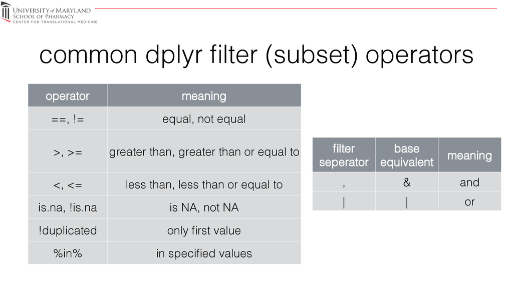
6. common dplyr filter (subset) operators! operator! meaning! ==, !=! equal, not equal! >, >=! greater than, greater than or equal to! <, <=! less than, less than or equal to! is.na, !is.na! is NA, not NA! !duplicated! only first value! %in%! in specified values! filter seperator! base equivalent! meaning! ,! &! and! |! |! or!
7. ID! GENDER! WT! 1! MALE! 70! 2! MALE! 76! 3! FEMALE! 60! 4! MALE! 64! 5! FEMALE! 68! filter(df, ID %in% c(1, 3, 5)) ID! GENDER! WT! 1! MALE! 70! 3! FEMALE! 60! 5! FEMALE! 68!
8. ID! GENDER! WT! 1! MALE! 70! 2! MALE! 76! 3! FEMALE! 60! 4! MALE! 64! 5! FEMALE! 68! filter(df, GENDER == “MALE”, WT > 70) ID! GENDER! WT! 2! MALE! 76!
9. ID! GENDER! WT! 1! MALE! 70! 2! MALE! 76! 3! FEMALE! 60! 4! MALE! 64! 5! FEMALE! 68! filter(df, GENDER == “FEMALE” | WT < 70) ID! GENDER! WT! 3! FEMALE! 60! 4! MALE! 64! 5! FEMALE! 68!
10. chaining and grouped operations!
11. chaining with %>%!
12. split-apply-combine -> group_by! http://www.gregreda.com/2013/10/26/working-with-pandas-dataframes/
13. dplyr verbs! Verb! Usage! filter! Keep matching row criteria! summarize! reduces summary values calculated ! mutate! add new variables to existing data frame! select! select columns by name! arrange! reorder rows!
14. ID! GENDER! WT! 1! MALE! 70! 2! MALE! 76! 3! FEMALE! 60! 4! MALE! 64! 5! FEMALE! 68! df %>% summarize(meanWT = mean(WT)) meanWT! 67.6! summarize(df, meanWT = mean(WT))
15. ID! GENDER! WT! 1! MALE! 70! 2! MALE! 76! 3! FEMALE! 60! 4! MALE! 64! 5! FEMALE! 68! df %>% group_by(GENDER) %>% summarize(meanWT = mean(WT)) GENDER! meanWT! MALE! 70! FEMALE! 64!
16. ID! GENDER! WT! 1! MALE! 70! 2! MALE! 76! 3! FEMALE! 60! 4! MALE! 64! 5! FEMALE! 68! df %>% group_by(GENDER) %>% summarize(meanWT = mean(WT), n = n()) GENDER! meanWT! n! MALE! 70! 3! FEMALE! 64! 2!
17. dplyr verbs! Verb! Usage! filter! Keep matching row criteria! summarize! reduces summary values calculated ! mutate! add new variables to existing data frame! select! select columns by name! arrange! reorder rows!
18. ID! GENDER! WT! 1! MALE! 70! 2! MALE! 76! 3! FEMALE! 60! 4! MALE! 64! 5! FEMALE! 68! df %>% mutate(meanWT = mean(WT)) ID! GENDER! WT! meanWT! 1! MALE! 70! 67.6! 2! MALE! 76! 67.6! 3! FEMALE! 60! 67.6! 4! MALE! 64! 67.6! 5! FEMALE! 68! 67.6!
19. ID! GENDER! WT! 1! MALE! 70! 2! MALE! 76! 3! FEMALE! 60! 4! MALE! 64! 5! FEMALE! 68! df %>% group_by(GENDER) %>% mutate(meanWT = mean(WT)) ID! GENDER! WT! meanWT! 1! MALE! 70! 70! 2! MALE! 76! 70! 3! FEMALE! 60! 64! 4! MALE! 64! 70! 5! FEMALE! 68! 64!
20. ID! GENDER! WT! 1! MALE! 70! 2! MALE! 76! 3! FEMALE! 60! 4! MALE! 64! 5! FEMALE! 68! df %>% group_by(GENDER) %>% mutate(meanWT = mean(WT), mWT_LB = meanWT*2.2) ID! GENDER! WT! meanWT! mWT_LB! 1! MALE! 70! 70! 154! 2! MALE! 76! 70! 154! 3! FEMALE! 60! 64! 140.8! 4! MALE! 64! 70! 154! 5! FEMALE! 68! 64! 140.8!
21. ID! GENDER! WT! 1! MALE! 70! 2! MALE! 76! 3! FEMALE! 60! 4! MALE! 64! 5! FEMALE! 68! df %>% mutate(ISM = ifelse(GENDER == “MALE”, 1, 0)) ID! GENDER! WT! ISM! 1! MALE! 70! 1! 2! MALE! 76! 1! 3! FEMALE! 60! 0! 4! MALE! 64! 1! 5! FEMALE! 68! 0!
22. dplyr verbs! Verb! Usage! filter! Keep matching row criteria! summarize! reduces summary values calculated ! mutate! add new variables to existing data frame! select! select columns by name! arrange! reorder rows!
23. ID! GENDER! WT! meanWT! 1! MALE! 70! 67.6! 2! MALE! 76! 67.6! 3! FEMALE! 60! 67.6! 4! MALE! 64! 67.6! 5! FEMALE! 68! 67.6! df2 %>% select(ID, WT) ID! WT! 1! 70! 2! 76! 3! 60! 4! 64! 5! 68!
24. ID! GENDER! WT! meanWT! 1! MALE! 70! 67.6! 2! MALE! 76! 67.6! 3! FEMALE! 60! 67.6! 4! MALE! 64! 67.6! 5! FEMALE! 68! 67.6! df2 %>% select(GENDER:meanWT) GENDER! WT! meanWT! MALE! 70! 67.6! MALE! 76! 67.6! FEMALE! 60! 67.6! MALE! 64! 67.6! FEMALE! 68! 67.6!
25. function! meaning! example! columns selected! starts_with! names start with! starts_with(“WEIGHT”))! WEIGHT, WEIGHT_KG! ends_with! names ends with! ends_with(“GHT”)! WEIGHT, MEAN_WEIGHT, HEIGHT! contains! names contains! contains(“EI”)! WEIGHT, WEIGHT_KG, MEAN_WEIGHT, HEIGHT! matches! regular expression matching! matches(“_”)! WEIGHT_KG, MEAN_WEIGHT! num_range! specify range of columns with consistent names with numeric suffix! num_range(“OCC”,1:3)! OCC1, OCC2, OCC3! test_select <- data.frame(“WEIGHT” =0, "WEIGHT_KG"=0, " " ""MEAN_WEIGHT"=0, “OCC1"=0, "OCC2"=0, ! " " ""OCC3"=0, "OCC4"=0, “HEIGHT"=0)! df %>% select(function())! WEIGHT! WEIGHT_KG! MEAN_WEIGHT! OCC1! OCC2! OCC3! OCC4! HEIGHT! df with the following columns:! test_select %>% select(starts_with(“WEIGHT”))! test_select %>% select(matches(“_”))! test_select %>% select(num_range(“OCC”, 1:3)!
26. ID! GENDER! WT! meanWT! 1! MALE! 70! 67.6! 2! MALE! 76! 67.6! 3! FEMALE! 60! 67.6! 4! MALE! 64! 67.6! 5! FEMALE! 68! 67.6! df2 %>% select(ID, WEIGHT = WT) ID! WEIGHT! 1! 70! 2! 76! 3! 60! 4! 64! 5! 68!
27. dplyr verbs! Verb! Usage! filter! Keep matching row criteria! summarize! reduces summary values calculated ! mutate! add new variables to existing data frame! select! select columns by name! arrange! reorder rows!
28. ID! GENDER! WT! 1! MALE! 70! 2! MALE! 76! 3! FEMALE! 60! 4! MALE! 64! 5! FEMALE! 68! ID! GENDER! WT! 3! FEMALE! 60! 4! MALE! 64! 5! FEMALE! 68! 1! MALE! 70! 2! MALE! 76! df %>% arrange(WT) lowest weight! highest weight!
29. ID! GENDER! WT! 1! MALE! 70! 2! MALE! 76! 3! FEMALE! 60! 4! MALE! 64! 5! FEMALE! 68! ID! GENDER! WT! 2! MALE! 76! 1! MALE! 70! 5! FEMALE! 68! 4! MALE! 64! 3! FEMALE! 60! df %>% arrange(desc(WT)) lowest weight! highest weight!
30. ID! TIME! AMT! MDV! 1! 0! 0! 0! 2! 0! 0! 0! 1! 1! 0! 0! 2! 1! 0! 0! 1! 2! 0! 0! 2! 2! 0! 0! 1! 0! 100! 1! 2! 0! 100! 1! * expand.grid is a very handy function for generating permutations! dosing_df <- data.frame(ID = 1:2, TIME =0, AMT = 100, MDV = 1) sample_df <- data.frame(expand.grid(ID = 1:2, TIME = seq(0, 2, 1), AMT = 0, MDV = 0) df3 <- rbind(sample_df, dosing_df) * MDV = missing dependent variable - a nonmem-style flag column! df3
31. ID! TIME! AMT! MDV! 1! 0! 0! 0! 2! 0! 0! 0! 1! 1! 0! 0! 2! 1! 0! 0! 1! 2! 0! 0! 2! 2! 0! 0! 1! 0! 100! 1! 2! 0! 100! 1! ID! TIME! AMT! MDV! 1! 0! 0! 0! 1! 0! 100! 1! 1! 1! 0! 0! 1! 2! 0! 0! 2! 0! 0! 0! 2! 0! 100! 1! 2! 1! 0! 0! 2! 2! 0! 0! df3 %>% arrange(ID, TIME)
32. ID! TIME! AMT! MDV! 1! 0! 0! 0! 2! 0! 0! 0! 1! 1! 0! 0! 2! 1! 0! 0! 1! 2! 0! 0! 2! 2! 0! 0! 1! 0! 100! 1! 2! 0! 100! 1! ID! TIME! AMT! MDV! 1! 0! 100! 1! 1! 0! 0! 0! 1! 1! 0! 0! 1! 2! 0! 0! 2! 0! 100! 1! 2! 0! 0! 0! 2! 1! 0! 0! 2! 2! 0! 0! df3 %>% arrange(ID, TIME, desc(MDV))
33. dplyr joins!
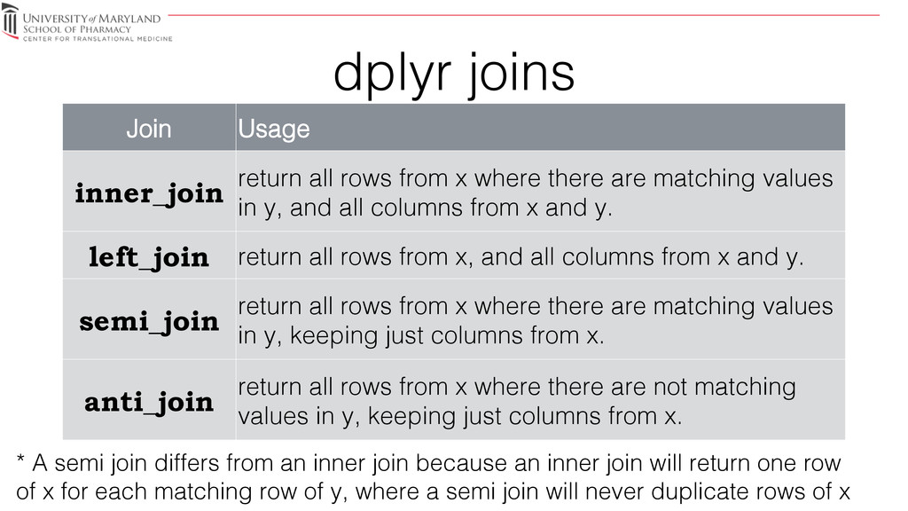
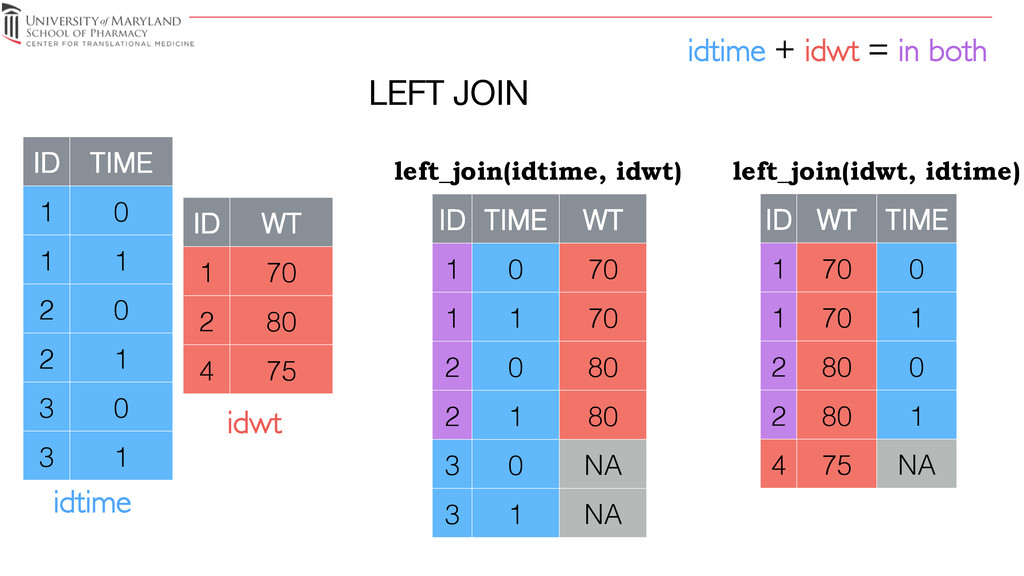
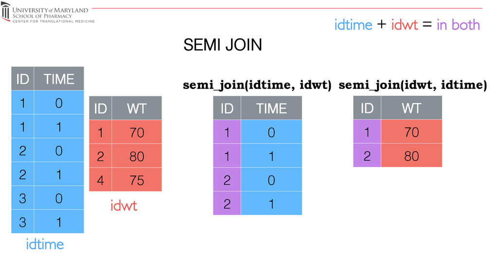
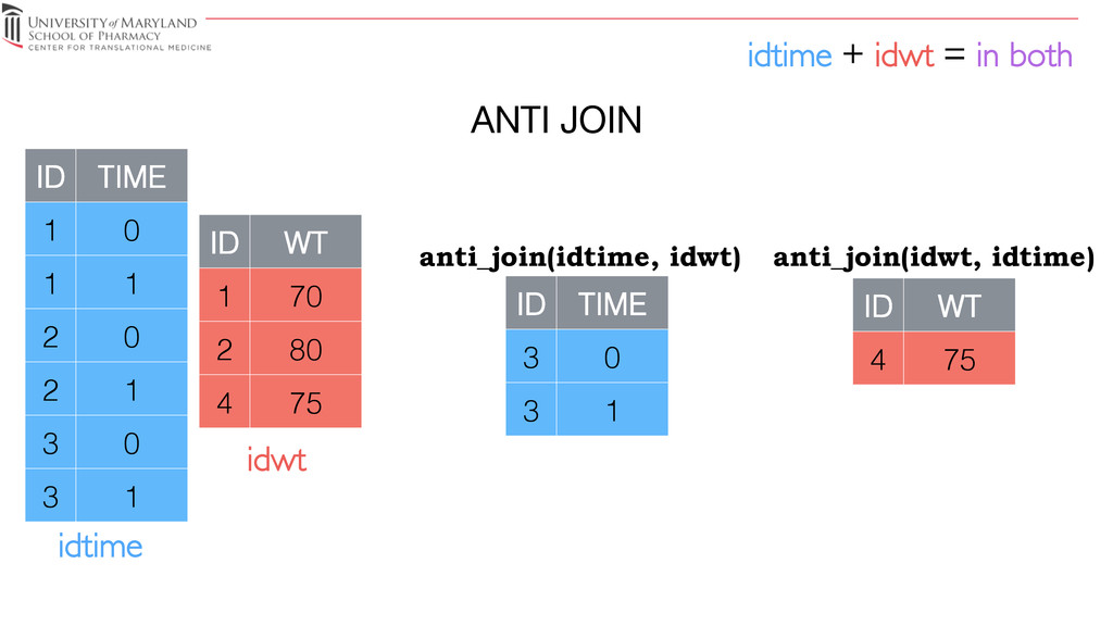
34. dplyr joins! Join! Usage! inner_join return all rows from x where there are matching values in y, and all columns from x and y.! left_join return all rows from x, and all columns from x and y.! semi_join return all rows from x where there are matching values in y, keeping just columns from x.! anti_join return all rows from x where there are not matching values in y, keeping just columns from x.! * A semi join differs from an inner join because an inner join will return one row of x for each matching row of y, where a semi join will never duplicate rows of x!
35. ID! TIME! 1! 0! 1! 1! 2! 0! 2! 1! 3! 0! 3! 1! idtime <- data.frame(expand.grid(ID = as.numeric(1:3), TIME = c(0,1))) %>% arrange(ID) idwt <- data.frame(ID = c(1, 2, 4), WT = c(70, 80, 75)) ID! WT! 1! 70! 2! 80! 4! 75! idtime idwt join syntax:! specific_join(x_dataframe, y_dataframe)!
36. INNER JOIN! ID! TIME! WT! 1! 0! 70! 1! 1! 70! 2! 0! 80! 2! 1! 80! ID! WT! TIME! 1! 70! 0! 1! 70! 1! 2! 80! 0! 2! 80! 1! idtime + idwt = in both inner_join(idtime, idwt) inner_join(idwt, idtime) ID! TIME! 1! 0! 1! 1! 2! 0! 2! 1! 3! 0! 3! 1! ID! WT! 1! 70! 2! 80! 4! 75! idtime idwt
37. ID! TIME! WT! 1! 0! 70! 1! 1! 70! 2! 0! 80! 2! 1! 80! 3! 0! NA! 3! 1! NA! ID! WT! TIME! 1! 70! 0! 1! 70! 1! 2! 80! 0! 2! 80! 1! 4! 75! NA! idtime + idwt = in both left_join(idtime, idwt) left_join(idwt, idtime) ID! TIME! 1! 0! 1! 1! 2! 0! 2! 1! 3! 0! 3! 1! ID! WT! 1! 70! 2! 80! 4! 75! idtime idwt LEFT JOIN!
38. ID! TIME! 1! 0! 1! 1! 2! 0! 2! 1! 3! 0! 3! 1! ID! WT! 1! 70! 2! 80! 4! 75! idtime idwt ID! TIME! 1! 0! 1! 1! 2! 0! 2! 1! ID! WT! 1! 70! 2! 80! idtime + idwt = in both semi_join(idtime, idwt) semi_join(idwt, idtime) SEMI JOIN!
39. ID! TIME! 1! 0! 1! 1! 2! 0! 2! 1! 3! 0! 3! 1! ID! WT! 1! 70! 2! 80! 4! 75! idtime idwt idtime + idwt = in both anti_join(idtime, idwt) anti_join(idwt, idtime) ID! TIME! 3! 0! 3! 1! ID! WT! 4! 75! ANTI JOIN!