Titan Transients, Inter-Corpora Correlations, and LLM Scalability

While benchmarking its ChatGPT LLMs internally, OpenAI researchers noticed
that after a significant amount of computational effort on a given size LLM, there was no improvement in Test Loss error reduction. Instead, the loss curve takes on a reverse-S shape or sigmoidal characteristic where the loss eventually remains constant at the foot of the S.
To combat this limitation, larger LLM instances—containing decades more neu-
ral net connections—were invoked to further reduce the Test Loss. However, that resulted in a sequence of successively lower sigmoidal curves that appear to fall on a descending line, which they called the ”compute-efficient frontier” (CEF). The CEF bound raised concerns that it might constitute a universal constraint on the scalability of all LLM systems.
This talk presents a model of LLM computational dynamics, based on the Univer-
sal Scalability Law, that provides a framework for understanding the CEF. The USL defines bistable minima in the tokenized neural net landscape.
This talk explains:
1. Why all training loss curves have a sigmoidal characteristic
2. Why the observed CEF constraint exists
3. What the CEF correlation means for LLM scalability
More details have been published in reference [1].

Transcript

1. Titan Transients, Inter-Corpora Correlations, and LLM Scalability Ghosts in the Machine Dr. Neil J. Gunther Performance Dynamics Research INFORMS: AI & Decision Intelligence Summit San José State University San José, California October 2, 2026 © 2026 Performance Dynamics Research Titan Transients, Inter-Corpora Correlations, and LLM Scalability October 2, 2026 1 / 29
2. Abstract While benchmarking its ChatGPT LLMs internally, OpenAI researchers noticed that after a significant amount of computational effort on a given size LLM, there was no improvement in Test Loss error reduction. Instead, the loss curve takes on a reverse-S shape or sigmoidal characteristic where the loss eventually remains constant at the foot of the S. To combat this limitation, larger LLM instances—containing decades more neural net connections—were invoked to further reduce the Test Loss. However, that resulted in a sequence of successively lower sigmoidal curves that appear to fall on descending line, which they called the ”compute-efficient frontier” (CEF). The CEF bound raised concerns that it might constitute a universal constraint on the scalability of all LLM systems. This talk presents a model of LLM computational dynamics, based on the Universal Scalability Law, that provides a framework for understanding the CEF. The USL defines bistable minima in the tokenized neural net landscape. This talk explains: 1 Why all training loss curves have a sigmoidal characteristic 2 Why the observed CEF constraint exists 3 What the CEF correlation means for LLM scalability More details have been published in [1]. © 2026 Performance Dynamics Research Titan Transients, Inter-Corpora Correlations, and LLM Scalability October 2, 2026 2 / 29
3. We Don’t Know Why Outline 1 We Don’t Know Why 2 Bistable Queues 3 Titan Transients 4 The Final Frontier 5 Conclusion 6 References © 2026 Performance Dynamics Research Titan Transients, Inter-Corpora Correlations, and LLM Scalability October 2, 2026 3 / 29
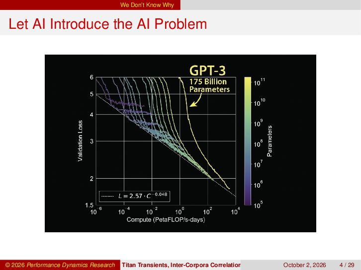
4. We Don’t Know Why Let AI Introduce the AI Problem © 2026 Performance Dynamics Research Titan Transients, Inter-Corpora Correlations, and LLM Scalability October 2, 2026 4 / 29
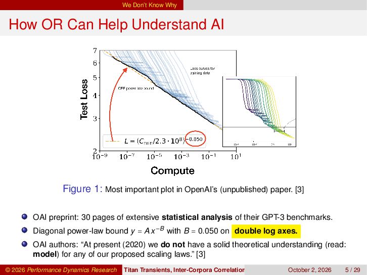
5. We Don’t Know Why How OR Can Help Understand AI Figure 1: Most important plot in OpenAI’s (unpublished) paper. [3] OAI preprint: 30 pages of extensive statistical analysis of their GPT-3 benchmarks. Diagonal power-law bound y = A x −B with B = 0.050 on double log axes. OAI authors: “At present (2020) we do not have a solid theoretical understanding (read: model) for any of our proposed scaling laws.” [3] © 2026 Performance Dynamics Research Titan Transients, Inter-Corpora Correlations, and LLM Scalability October 2, 2026 5 / 29
6. We Don’t Know Why Our Queueing Theory Approach 1 Bistable queues 2 3D Cost function 3 Titan transients 4 Relate to the CEF 5 Interpret the CEF Lightning Talk All mathematical analysis has been suppressed in the interest of time. © 2026 Performance Dynamics Research Titan Transients, Inter-Corpora Correlations, and LLM Scalability October 2, 2026 6 / 29
7. Bistable Queues Outline 1 We Don’t Know Why 2 Bistable Queues 3 Titan Transients 4 The Final Frontier 5 Conclusion 6 References © 2026 Performance Dynamics Research Titan Transients, Inter-Corpora Correlations, and LLM Scalability October 2, 2026 7 / 29
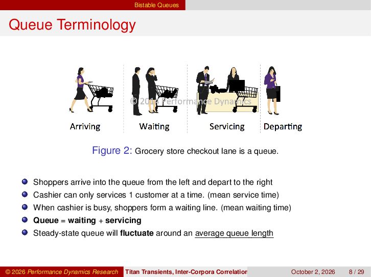
8. Bistable Queues Queue Terminology Figure 2: Grocery store checkout lane is a queue. Shoppers arrive into the queue from the left and depart to the right Cashier can only services 1 customer at a time. (mean service time) When cashier is busy, shoppers form a waiting line. (mean waiting time) Queue = waiting + servicing Steady-state queue will fluctuate around an average queue length © 2026 Performance Dynamics Research Titan Transients, Inter-Corpora Correlations, and LLM Scalability October 2, 2026 8 / 29
9. Bistable Queues Universal Scalability Law or USL X(N) Out[ ] = 0 50 100 150 200 N N: number of customers or processes in the system X (N): queue throughput or departure rate The three Cs: 1 Concurrency (linear-rising parallelism) 2 Contention (queueing asymptote) 3 Coherency (data exchange or pre-service sorting degradation) © 2026 Performance Dynamics Research Titan Transients, Inter-Corpora Correlations, and LLM Scalability October 2, 2026 9 / 29
10. Bistable Queues USL Bistable Queue Out[ ] = Figure 3: Aggregated bistable queue. Multi-GPU service facility (blue disk) with waiting tokens (red blocks). Mean arrival rate (red curve) and departure rate (blue). Two mean lengths queue Nopt and Nslow . Stability points: 1 Nopt — stable optimal queue (left) 2 Ncrit — unstable queue length (center) 3 Nslow — stable congested queue (right) © 2026 Performance Dynamics Research Titan Transients, Inter-Corpora Correlations, and LLM Scalability October 2, 2026 10 / 29
11. Bistable Queues Out[ ] = Take the difference of red − blue © 2026 Performance Dynamics Research Titan Transients, Inter-Corpora Correlations, and LLM Scalability October 2, 2026 11 / 29
12. Bistable Queues Drift (b) Out[ ] = N Take the negative integral © 2026 Performance Dynamics Research Titan Transients, Inter-Corpora Correlations, and LLM Scalability October 2, 2026 11 / 29
13. Bistable Queues Cost (c) Out[ ] = N Nonlinear cost function © 2026 Performance Dynamics Research Titan Transients, Inter-Corpora Correlations, and LLM Scalability October 2, 2026 11 / 29
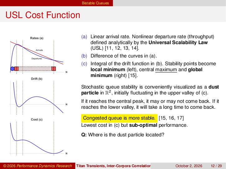
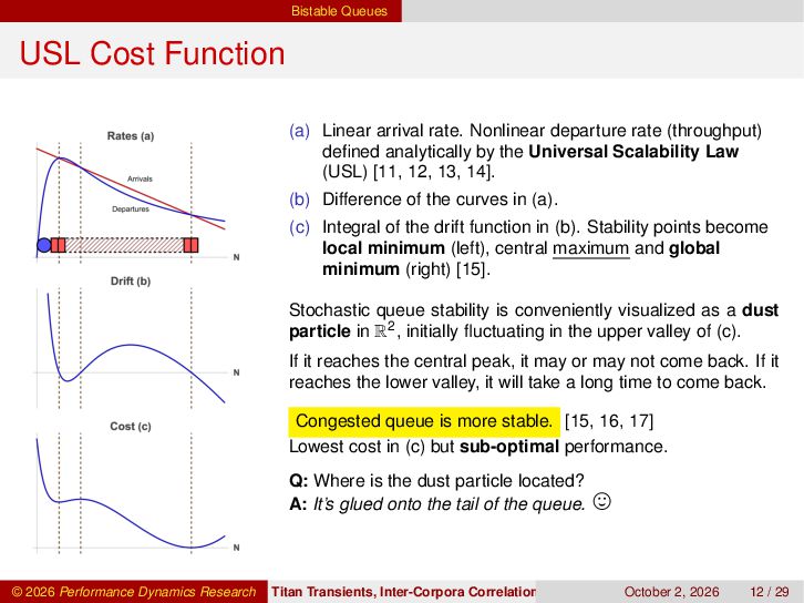
14. Bistable Queues USL Cost Function (a) Linear arrival rate. Nonlinear departure rate (throughput) defined analytically by the Universal Scalability Law (USL) [11, 12, 13, 14]. (b) Difference of the curves in (a). (c) Integral of the drift function in (b). Stability points become local minimum (left), central maximum and global minimum (right) [15]. Out[ ] = Stochastic queue stability is conveniently visualized as a dust particle in R2 , initially fluctuating in the upper valley of (c). If it reaches the central peak, it may or may not come back. If it reaches the lower valley, it will take a long time to come back. Congested queue is more stable. [15, 16, 17] Lowest cost in (c) but sub-optimal performance. Q: Where is the dust particle located? © 2026 Performance Dynamics Research Titan Transients, Inter-Corpora Correlations, and LLM Scalability October 2, 2026 12 / 29
15. Bistable Queues USL Cost Function (a) Linear arrival rate. Nonlinear departure rate (throughput) defined analytically by the Universal Scalability Law (USL) [11, 12, 13, 14]. (b) Difference of the curves in (a). (c) Integral of the drift function in (b). Stability points become local minimum (left), central maximum and global minimum (right) [15]. Out[ ] = Stochastic queue stability is conveniently visualized as a dust particle in R2 , initially fluctuating in the upper valley of (c). If it reaches the central peak, it may or may not come back. If it reaches the lower valley, it will take a long time to come back. Congested queue is more stable. [15, 16, 17] Lowest cost in (c) but sub-optimal performance. Q: Where is the dust particle located? A: It’s glued onto the tail of the queue. , © 2026 Performance Dynamics Research Titan Transients, Inter-Corpora Correlations, and LLM Scalability October 2, 2026 12 / 29
16. Titan Transients Outline 1 We Don’t Know Why 2 Bistable Queues 3 Titan Transients 4 The Final Frontier 5 Conclusion 6 References © 2026 Performance Dynamics Research Titan Transients, Inter-Corpora Correlations, and LLM Scalability October 2, 2026 13 / 29
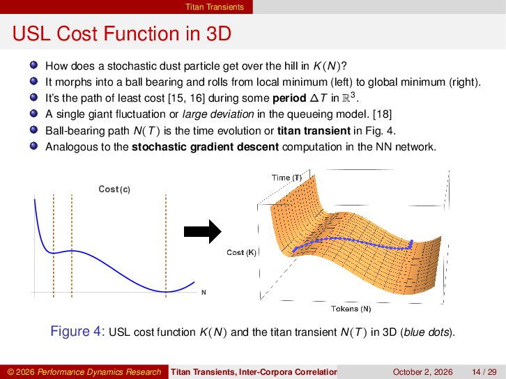
17. Titan Transients USL Cost Function in 3D How does a stochastic dust particle get over the hill in K (N)? It morphs into a ball bearing and rolls from local minimum (left) to global minimum (right). It’s the path of least cost [15, 16] during some period ∆T in R3 . A single giant fluctuation or large deviation in the queueing model. [18] Ball-bearing path N(T ) is the time evolution or titan transient in Fig. 4. Analogous to the stochastic gradient descent computation in the NN network. Cost (c) Out[ ] = Out[ ] = N Figure 4: USL cost function K (N) and the titan transient N(T ) in 3D (blue dots). © 2026 Performance Dynamics Research Titan Transients, Inter-Corpora Correlations, and LLM Scalability October 2, 2026 14 / 29
18. Titan Transients Titan Transient in 3D Out[ ] = Figure 5: Fig.4 oriented to match the LLM loss-compute curves in Fig. 1. N(T ) curve represents a huge fluctuation or titan transient N(T ) has characteristic sigmoidal shape of LLM loss functions N(T ) has to be calculated numerically in Fig. 5 N(T ) is the time-dependent queue length of LLM tokens, i.e., waiting + service © 2026 Performance Dynamics Research Titan Transients, Inter-Corpora Correlations, and LLM Scalability October 2, 2026 15 / 29
19. The Final Frontier Outline 1 We Don’t Know Why 2 Bistable Queues 3 Titan Transients 4 The Final Frontier 5 Conclusion 6 References © 2026 Performance Dynamics Research Titan Transients, Inter-Corpora Correlations, and LLM Scalability October 2, 2026 16 / 29
20. The Final Frontier USL Compute Frontier Out[ ] = Figure 6: Selected successive global USL cost minima (curves)—each rescaled by an order of magnitude—lie on the power-law bound Kmin (N) = A ⋅ N −B (pink plane). © 2026 Performance Dynamics Research Titan Transients, Inter-Corpora Correlations, and LLM Scalability October 2, 2026 17 / 29
21. The Final Frontier OAI Figure 1 Explained Out[ ] = Figure 7: View through the (K , T ) plane. Swivel Fig. 6 clockwise about its log K axis Schematic loss curves (blue lines) Thick arrows match the global USL minima (red lines) in Fig. 6 Flattened view through the (K , T ) plane © 2026 Performance Dynamics Research Titan Transients, Inter-Corpora Correlations, and LLM Scalability October 2, 2026 18 / 29
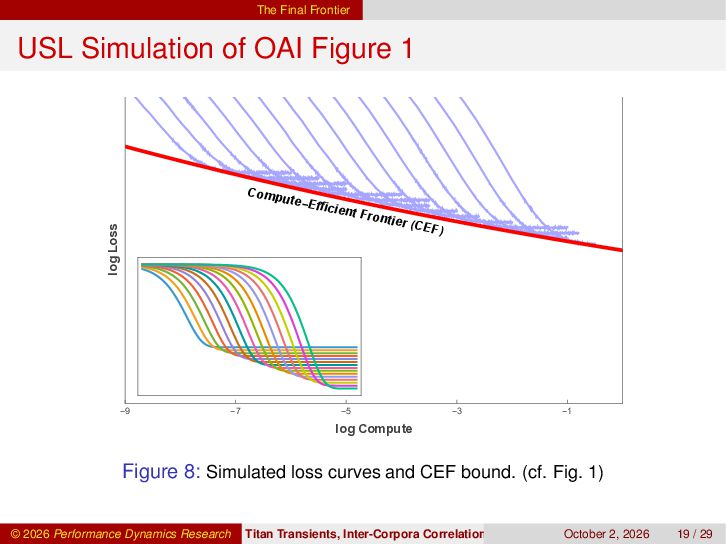
22. The Final Frontier USL Simulation of OAI Figure 1 Comp ute-E t Fron log Loss Out[ ] = fficien -9 -7 tier (C -5 EF) -3 -1 log Compute Figure 8: Simulated loss curves and CEF bound. (cf. Fig. 1) © 2026 Performance Dynamics Research Titan Transients, Inter-Corpora Correlations, and LLM Scalability October 2, 2026 19 / 29
23. Conclusion Outline 1 We Don’t Know Why 2 Bistable Queues 3 Titan Transients 4 The Final Frontier 5 Conclusion 6 References © 2026 Performance Dynamics Research Titan Transients, Inter-Corpora Correlations, and LLM Scalability October 2, 2026 20 / 29
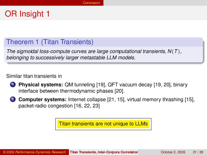
24. Conclusion OR Insight 1 Theorem 1 (Titan Transients) The sigmoidal loss-compute curves are large computational transients, N(T ), belonging to successively larger metastable LLM models. Similar titan transients in 1 Physical systems: QM tunneling [19], QFT vacuum decay [19, 20], binary interface between thermodynamic phases [20]. 2 Computer systems: Internet collapse [21, 15], virtual memory thrashing [15], packet-radio congestion [16, 22, 23] Titan transients are not unique to LLMs © 2026 Performance Dynamics Research Titan Transients, Inter-Corpora Correlations, and LLM Scalability October 2, 2026 21 / 29
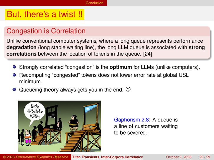
25. Conclusion But, there’s a twist !! Congestion is Correlation Unlike conventional computer systems, where a long queue represents performance degradation (long stable waiting line), the long LLM queue is associated with strong correlations between the location of tokens in the queue. [24] Strongly correlated “congestion” is the optimum for LLMs (unlike computers). Recomputing “congested” tokens does not lower error rate at global USL minimum. Queueing theory always gets you in the end. , Gaphorism 2.8: A queue is a line of customers waiting to be severed. © 2026 Performance Dynamics Research Titan Transients, Inter-Corpora Correlations, and LLM Scalability October 2, 2026 22 / 29
26. Conclusion Zipf’s Law ZipfLaw(x) 0.30 [ ] = PwrLaw(1.5, x) 0.25 exp(-x) 0.20 PwrLaw(0.5, x) 0.15 All continuous parametric dsns have exponential tails. (dashed curve) Zipf’s law for ranked context-free frequency counts of (English) words in a single corpus, i.e., B = 1 in A x −B (dashed red line) Zipf correlations are stronger than exponential tails 0.10 0.05 20 40 60 80 100 10 OpenAI’s exponent B = 0.05 (≪ 1) implies very strong correlations ( blue line) 1 0.100 [ ] = ZipfLaw(x) 0.010 PwrLaw(1.5, x) exp(-x) 0.001 PwrLaw(0.5, x) 10-4 PwrLaw(0.05, x) 1 5 10 © 2026 Performance Dynamics Research 50 100 Titan Transients, Inter-Corpora Correlations, and LLM Scalability October 2, 2026 23 / 29
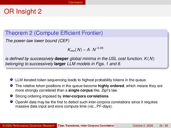
27. Conclusion OR Insight 2 Theorem 2 (Compute Efficient Frontier) The power-law lower bound (CEF) Kmin (N) = A ⋅ N −0.05 is defined by successively deeper global minima in the USL cost function, K (N) belonging to successively larger LLM models in Figs. 1 and 8. LLM iterated token sequencing leads to highest probability tokens in the queue. The relative token positions in the queue become highly ordered, which means they are more strongly correlated than a single corpus like, Zipf’s law. Strong ordering imposed by inter-corpora correlations. OpenAI data may be the first to detect such inter-corpora correlations since it requires massive data input and eons compute time (viz., PF-days). © 2026 Performance Dynamics Research Titan Transients, Inter-Corpora Correlations, and LLM Scalability October 2, 2026 24 / 29
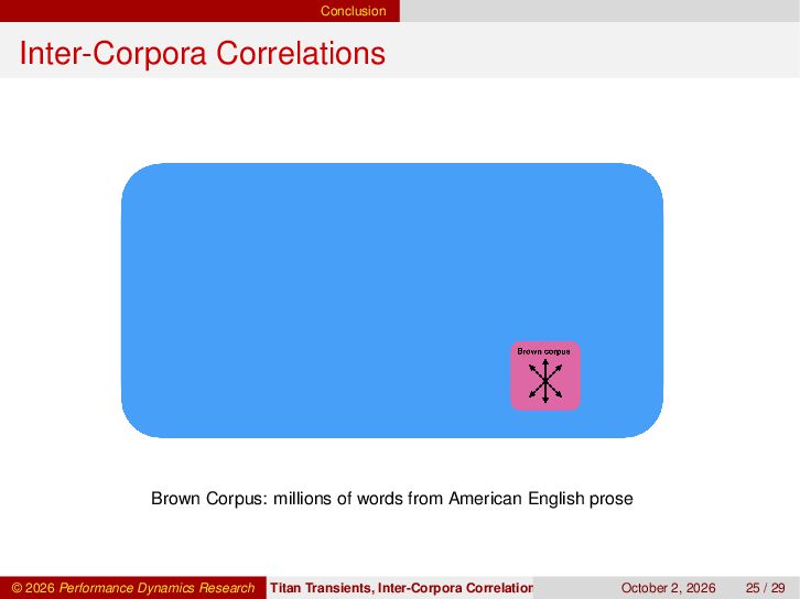
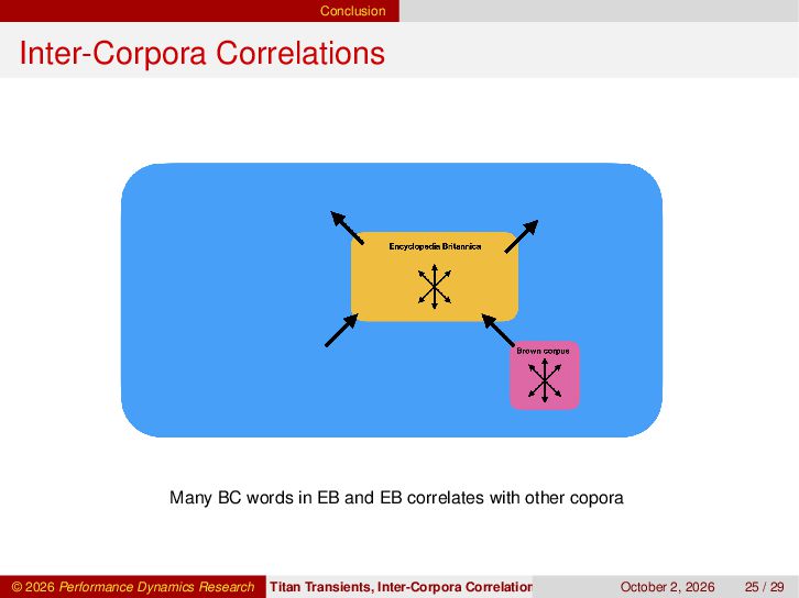
28. Conclusion Inter-Corpora Correlations Brown Corpus: millions of words from American English prose © 2026 Performance Dynamics Research Titan Transients, Inter-Corpora Correlations, and LLM Scalability October 2, 2026 25 / 29
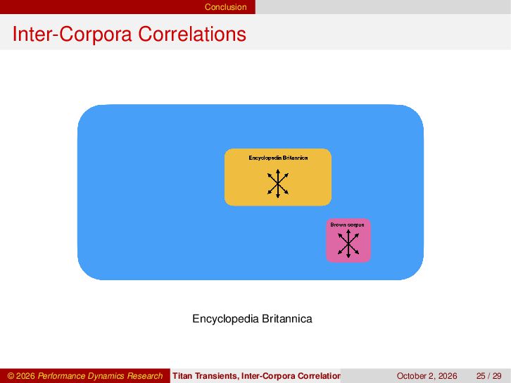
29. Conclusion Inter-Corpora Correlations Encyclopedia Britannica © 2026 Performance Dynamics Research Titan Transients, Inter-Corpora Correlations, and LLM Scalability October 2, 2026 25 / 29
30. Conclusion Inter-Corpora Correlations Many BC words in EB and EB correlates with other copora © 2026 Performance Dynamics Research Titan Transients, Inter-Corpora Correlations, and LLM Scalability October 2, 2026 25 / 29
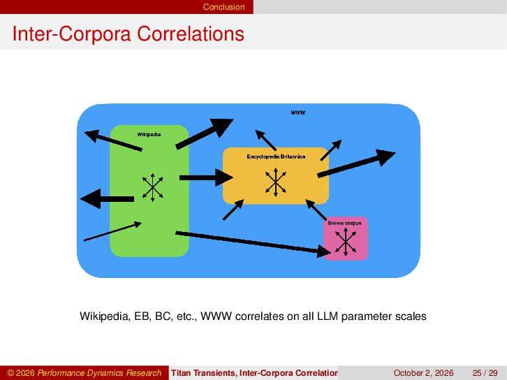
31. Conclusion Inter-Corpora Correlations Wikipedia, EB, BC, etc., WWW correlates on all LLM parameter scales © 2026 Performance Dynamics Research Titan Transients, Inter-Corpora Correlations, and LLM Scalability October 2, 2026 25 / 29
32. References Outline 1 We Don’t Know Why 2 Bistable Queues 3 Titan Transients 4 The Final Frontier 5 Conclusion 6 References © 2026 Performance Dynamics Research Titan Transients, Inter-Corpora Correlations, and LLM Scalability October 2, 2026 26 / 29
33. References References I [1] N.J. Gunther, “Titan Transients and LLM Scalability,” ACM Queue, Vol. 24, No. 3, July 22 (2026) [2] A. Vaswani, N. Shazeer, et al., “Attention Is All You Need, ” 31st Conference on Neural Information Processing Systems (NIPS), Long Beach, CA (2017) and online at arXiv (2023) [3] J. Kaplan, S. McCandlish, T. J. Henighan, et al., “Scaling Laws for Neural Language Models,” arXiv (2020) [4] M. Newman, “Power laws, Pareto distributions and Zipf’s law,”’ Contemporary Physics, 46(5), 323–351 (2005) [5] N. Maroney and N.J. Gunther, “Power Law Analysis of MagCloud Publications,” HP Labs Internal Technical Teport CW237032 (2011) [6] Welch Labs, “Can’t Cross This Line and We Don’t Know Why,” YouTube, September 13 (2024) [7] hampton—e/acc, “Have we discovered a fundamental law of nature for building intelligent systems?” Twitter/X, August 23 (2024) [8] E.D.Lasowska, J. Zahorjan, G.S. Graham, and K.C. Sevcik, Quantitative System Performance: Computer System Analysis Using Queueing Network Models, Engelwood Cliffs: Prentice-Hall (1984) [9] N.J. Gunther, Analyzing Computer System Performance with Perl::PDQ, 2nd Edition, Springer (2011) [10] P.J. Courtois, “Decomposability, Instabilities, and Saturation in Multiprogramming Systems”, Comm. ACM, No. 7, Vol.18, 371-377 (1975) [11] N.J. Gunther, Guerrilla Capacity Planning, Springer (2007) [12] J. Holtman and N.J. Gunther, “Getting in the Zone for Successful Scalability,” Proc. CMG Conference, Las Vegas, Nevada (2008) arXiv [13] N.J. Gunther, “A General Theory of Computational Scalability Based on Rational Functions,” arXiv (2008) [14] N.J. Gunther, How to Quantify Scalability: The Universal Scalability Law (USL), 27 Feb (2020) © 2026 Performance Dynamics Research Titan Transients, Inter-Corpora Correlations, and LLM Scalability October 2, 2026 27 / 29
34. References References II [15] N.J. Gunther, “Path Integrals for Computers,” Information Processing Letters, 32(1): 7-13 (1989) [16] N.J. Gunther and J.G. Shaw, ”Path Integral Evaluation of ALOHA Network Transients,” Information Processing Letters, 33(6): 289-295 (1990) [17] N.J. Gunther, “Bilinear Model of Blocking Transients in Large Circuit-Switching Networks,” In PERFORMANCE’90, Proceedings of the 14th IFIP WG 7.3 International Symposium on Computer Performance Modelling, Measurement and Evaluation, Edinburgh, Scotland, 12-14, September, Amsterdam: North-Holland, 175-189 (1990) [18] A. Ganesh, N. O’Connell and D. Wischik, Big Queues, Lecture Notes in Mathematics, Springer-Verlag, Heidelberg (2004) [19] S. Coleman, “The Uses of Instantons,” Chap. 7 in Aspects of Symmetry, Cambridge Univ. Press (1985) [20] N.J. Gunther, D.A. Nicole and D.J. Wallace, “Goldstone Modes in Vacuum Decay and First-Order Phase Transitions,” J. Phys. A. 13, 1755-1767 (1980) [21] V. Jacobson, “Congestion Avoidance and Control,” ACM SIGCOMM Computer Communication Review, Vol. 18, No. 4, 314-329, August (1988) [22] R.M. Metcalfe, “Steady-state Analysis of the a Slotted and Controlled ALOHA System with Blocking,” In Proc. VI Hawaii Conf. on System Sciences (1973) [23] R.M. Metcalfe and D.R. Boggs, “Ethernet: Distributed Packet Switching for Local Computer Networks,” Comm. ACM. 19(7): 395 (1976) [24] J.F. Brady and N.J. Gunther, “How to Emulate Web Traffic Using Standard Load Testing Tools,” Proc. CMG Conference, La Jolla, California, arXiv (2016) © 2026 Performance Dynamics Research Titan Transients, Inter-Corpora Correlations, and LLM Scalability October 2, 2026 28 / 29
35. References Questions? Thank you for your participation www.perfdynamics.com Castro Valley, California Twitter twitter.com/DrQz Facebook facebook.com/PerformanceDynamics Blog perfdynamics.blogspot.com Training perfdynamics.com/Classes Email info@perfdynamics.com © 2026 Performance Dynamics Research Titan Transients, Inter-Corpora Correlations, and LLM Scalability October 2, 2026 29 / 29